Probably Dance

I’m trying to get into neural networks. There have been a couple big breakthroughs in the field in recent years and suddenly my side project of messing around with programming languages seemed short sighted. It almost seems like we’ll have real AI soon and I want to be working on that. While making my first couple steps into the field it’s hard to keep that enthusiasm. A lot of the field is still kinda handwavy where when you want to find out why something is used the way it’s used, the only answer you can get is “because it works like this and it doesn’t work if we change it.”

At least that’s my first impression. Still just dipping my toes in. But there is one thing I am very impressed with: How much data neural networks can express in how few connections.

To illustrate let me draw a very simple neural network. It’s not a very interesting neural network, I’m just connecting inputs to outputs:

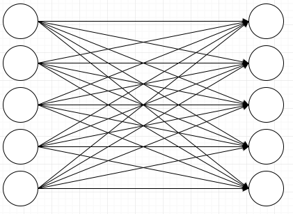
And now let’s say that I want to teach this neural network the following pattern: Whenever input 1 fires, fire output 2. When input 2 fires, fire output 3. When input 3 fires, fire output 4. When input 4 fires, fire output 5. Output 1 never gets fired and input 5 never gets fired. To do that you use an algorithm called back propagation and repeatedly tell the network what output you expect for a given input, but that is not what I want to talk about here. I want to talk about the results. I’ll make the connections that the network learns stronger, and the connections that the network doesn’t learn weaker:

What happened here is that the weights for some connections have increased, while the weights for most connections have decreased. I haven’t talked about weights yet. Weights are what neural networks learn. When we draw networks, the nodes seem more important. But what the network actually learns and stores are weights on the connections. In the picture above the thick lines have a weight of 1, the others have a weight of 0. (weights can also go negative, and they can go up arbitrarily high)

Hidden Layers

A simple network like the one above can learn simple patterns like this. If we want to learn more complex patterns, we have to create a network that has more layers. Let’s insert a layer with two neurons in the middle:

There are many possible behaviors for those neurons in the middle, and that is the part where most of the magic happens in neural networks. It seems like picking what goes there just requires experimentation and experience. A simple neuron would be the tanh neuron which does these three steps:

1. add up all of its inputs multiplied by their weights
2. calculate tanh() on the sum
3. fire the result to its outputs multiplied by their weights

Why tanh? Because it has a couple convenient properties, and it happens to work better than other functions that have the same properties. But mostly it’s “beause it works like this and it doesn’t work when we change it.”

If you count the number of connections on that last picture you will notice that there are fewer than there were in the first network. There were 5*5=25 at first, now there are 5*2*2=20. That reduction would be larger if I had more input and output nodes. For 10 nodes that reduction would be from 100 connections down to 40 when inserting two nodes in the middle. That’s where the compression in the title of this blog post comes from.

The question is whether we can still represent the original pattern in this new representation. To show why that is not obvious, I’ll explain why it doesn’t work if you just have one middle neuron:

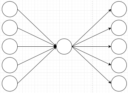
If I initialize the weights on here so that the first node fires the second output, all nodes will fire the second output:

That one node in the middle messes up the ability for my network to learn my very simple rule. This network can not learn different behaviors for different input nodes because they all have to go through that one node in the middle. Remember that the node in the middle just adds all of its inputs, so it can not have different behaviors depending on which input it receives. The information of where a value came from gets lost in the summation.

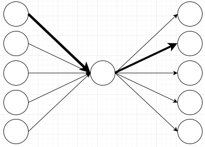
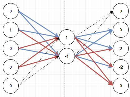
So how many nodes do I need to put into the middle to still be able to learn my rule? In real neural networks you usually put hundreds of nodes into that middle layer, but what is the minimal number to learn my pattern? Before I get to the answer I need to explain one more type of neuron that enables my compression: The softmax layer. If I make my output layer a softmax layer, that means that it will look at all the activations on that layer, and that it will only fire the output with the highest activation. That’s where the “max” in the softmax comes from: It fires the max node. The “soft” part is also very important in other contexts because a softmax layer can fire more than one output, but in my case it will only ever fire one output so we’ll stay with this explanation. If I make my middle layer a tanh layer and my output layer a softmax layer, I can represent my pattern just by having two nodes in the middle:

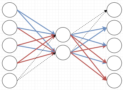
Here I’ve made lines with positive weights blue, and lines with negative weights red. This means that if for example the first input fires, I will get these values on the nodes:

The first node activates both the middle nodes. That activates the second output node with weight two. The next two nodes are canceled out because they receive a positive weight from one of the middle nodes and a negative weight from the other. The last node is activated with weight -2. If I then run softmax on this only the top node will fire. Meaning the bottom node will not fire a negative output. Softmax suppresses everything except for the most active node.

This is a little bit simplified, because the tanh layer doesn’t give out nice round numbers and the softmax layer wants bigger numbers, but those complications are not necessary to understand what’s going on, so I’ll keep the numbers in this blog post simple. (the real weights in my test code are +9 and -9 on the connections going from the input layer to the middle layer, and +26 and -26 on the connections going from the middle layer to the output layer. I don’t know why those numbers specifically, that’s just where the network decided to stabilize)

Let’s quickly run through this for the other three cases as well:

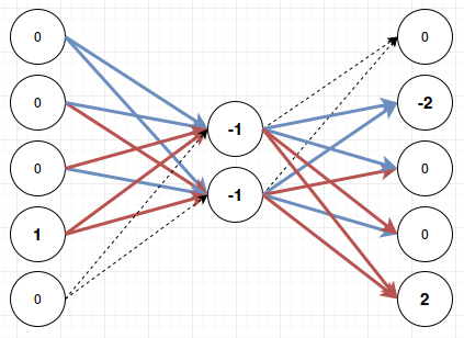
As you can see there is always one clear winner and then the softmax layer at the end will make sure that only that one fires and the other outputs remain quiet. When I first saw this behavior I was quite impressed. In fact I saw this behavior on a network with eleven inputs, eleven outputs and just two middle nodes. Can you think of how the above layer would work with eleven inputs? It seems like there’s only four possible combinations for these weights and we’ve used all of them, right? You’re underestimating neural networks. It’s quite impressive how they will try to squeeze any pattern that you throw at them into what’s available. For eleven inputs and eleven outputs it looks like this:

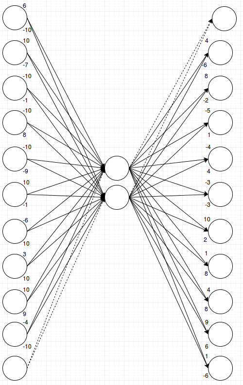
That is a lot of connections and a lot of numbers. The network has now decided to make some connections stronger and other connections weaker. I couldn’t keep using colors and line-style to visualize different strengths because now there are a lot of different values. Whenever I tried to simplify and not use numbers I’d break the network. So instead I just show the numbers. The upper number on each node is the weight of the connection to/from the upper node in the middle layer, and the lower number is the weight of the connection to/from the lower node in the middle layer.

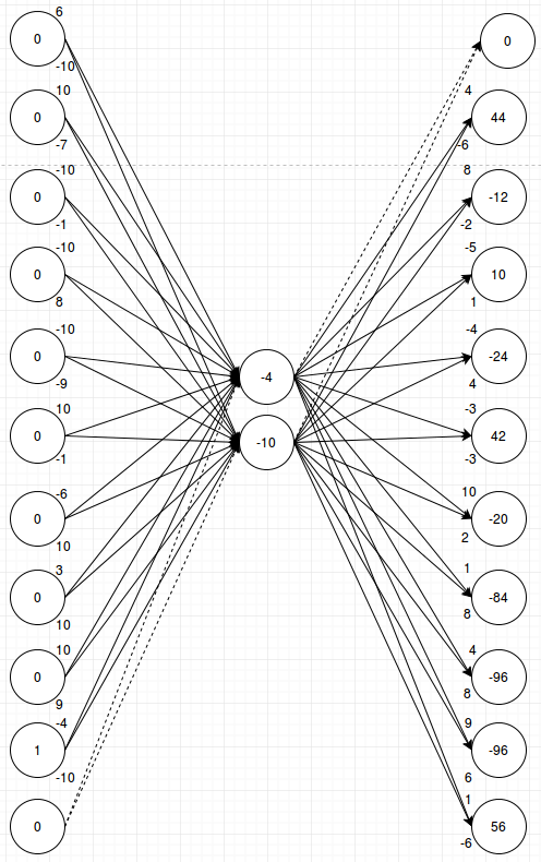
Let’s walk through a random example and see how it works:

The node with the largest output value (72 = -10 * -4 + 8 * 4) is the one we want to fire, and softmax will select that. In this picture I’m just multiplying the numbers linearly because the weights on the left actually already have tanh applied (and were then multiplied by 10 to get them into the range -10 to 10 which is slightly nicer for pictures than the range -1 to 1). I can do that in this case since I only ever fire one input. And if I can just do linear math the example is easier to follow.

I’ll post a second example to show that the weights will activate the desired output for any input:

Here also for my given input n, output n+1 had the highest value at the end and softmax will make that output fire. You could go through a couple more examples and convince yourself that this network has learned the pattern that I want it to learn.

I don’t know about you, but I think this is quite impressive. For the small first network I think I could have figured out how to put the numbers in manually. (once you know the trick that the nodes can cancel each other out it’s easy) For all the connections on the larger network you would have to be very good at balancing these weights, and I honestly don’t think I could have done this by hand. The neural network however seems to just figure this out. Or rather: it figures this out if you use a tanh layer in the middle and a softmax layer at the end. If you don’t, it will stop working.

Since I’m using real numbers now I might as well explain how softmax works. Softmax uses the number at the end as an exponent and then normalizes the column afterwards. If I use 2^x it should be obvious that 2^56, the highest number, is a lot bigger than 2^44, the next highest number. If I have 2^56 in the column and I normalize it, all the other activations will go very close to zero and the output that I want to fire will be close to 1. Also by using an exponent I get no negative numbers. 2^-96 is just a number that’s very close to zero. The standard is to use e^x instead of 2^x, and I also use that, it’s just that as a programmer I find it easier to explain and easier to understand using powers of two.

How This Works

With that information I can give a bit of an intuition why this happens to work if you use tanh and softmax: When using softmax, the connections can keep on improving the chance of their desired output just by making their own weights bigger. In fact since I just used linear math in my explanation above and didn’t need to run tanh() on anything, couldn’t softmax have learned those weighs even without using a tanh layer? In theory it could, but in practice it will keep on bumping up the numbers to get small improvements and you will very quickly overflow floating point numbers. The tanh layer in the middle is then just responsible for keeping the numbers small: it clamps its outputs to the range -1 to 1, and the inputs won’t grow past a certain point either because at some point a bigger number just means that the output goes from 0.995 to 0.997. But since they can usually still get a small improvement you don’t lose that nice property of softmax where neurons can keep on edging out small improvements over each other.

So if you just use softmax your weights will explode and if you just use tanh your weights will stagnate too soon before a good solution emerges. If you use both you get nice greedy behavior where the connections keep on looking for better solutions, but you also keep the weights from exploding.

Now all I’ve shown is that my network can learn the rule that when input n fires, it needs to fire output n+1. It should be easy to see that just by creating a different permutation of the weights of the connections I can teach my network that for any input neuron x, it should fire any other output neuron y. The impressive part is that without the middle layer I would have needed 11*11 = 121 connections to have a network that can learn any combination, and with that middle layer I can do it in only 11*2*2 = 44 connections.

Eleven inputs and outputs is close to the limit for what you can do with two nodes in the middle. If you ask it to do much more the weights will fluctuate and they will keep on stepping on each others toes. But with three nodes in the middle I can learn these patterns for something like thirty inputs and outputs, and with four nodes, I can learn direct connections for more than a hundred inputs and outputs. It doesn’t grow linearly because the number of combinations doesn’t grow linearly. Luckily the back propagation algorithm scales with the number of connections, not with the number of combinations. So with a linear increase in computation cost I get a super-linear increase in the amount of stuff I can learn.

Outlook and Conclusions

I’m still just getting started with neural networks, and real networks look nothing like my tiny examples above. I don’t know how many neurons people actually use nowadays, but even small examples talk about hundreds of neurons. At that point it’s more difficult to understand what your network has learned. You can’t visualize it as easily as the above pictures. In fact even the eleven neuron picture is difficult to understand because you can’t just look at the strong connections. Even the weak connections are important. If that middle layer had 700 neurons, then good luck getting a picture of which connections are actually important. Maybe a bunch of weak connections add up to build the output you wanted and one random strong connection suppresses all the unwanted outputs that you didn’t want.

But I hope I have given you an intuition for how neural networks can compress patterns in few weights. They use the full range of the weights to the point where a connection activated with a strong input can mean something entirely different than the same connection activated with a weak input. And best of all I didn’t have to teach them to do this. They just start behaving like this if you force them to express a complex pattern in few connections.