Probably Dance

I recently learned how radix sort works, and in hindsight it’s weird that I never really learned about it before, and that it doesn’t seem to be widely used. In this blog post I claim that std::sort should use radix sort for large arrays, and I will provide a simple implementation that does that.

But first an explanation of what radix sort is: Radix sort is a O(n) sorting algorithm working on integer keys. I’ll explain below how it works, but the claim that there’s an O(n) searching algorithm was surprising to me the first time that I heard it. I always thought there were proofs that sorting had to be O(n log n). Turns out sorting has to be O(n log n) if you use the comparison operator to sort. Radix sort does not use the comparison operator, and because of that it can be faster.

The other reason why I never looked into radix sort is that it only works on integer keys. Which is a huge limitation. Or so I thought. Turns out all this means is that your struct has to be able to provide something that acts somewhat like an integer. Radix sort can be extended to floats, pairs, tuples and std::array. So if your struct can provide for example a std::pair<bool, float> and use that as a sort key, you can sort it using radix sort.

I actually do this somewhat often when I write C++ code nowadays. One recent example was that I had to sort enemies in a game that I was working on. I wanted to sort enemies by distance, but I wanted all enemies that were already fighting with the player to come first. So here is what the comparison function looked like:

bool operator<(const Enemy & a, const Enemy & b)
{
    return std::make_tuple(!IsInCombat(a), DistanceToPlayer(a))
         < std::make_tuple(!IsInCombat(b), DistanceToPlayer(b));
}

Using that comparison operator will sort the enemies so that all enemies that are in combat with the player come first, (and they’re sorted by distance) and then there will be all enemies that are not in combat with the player. (also sorted by distance)

Except that by using this comparison operator I have to use an O(n log n) sorting algorithm. But you can use radix sort to sort tuples, so I could sort this in O(n). All I have to do is provide this function

auto sort_key(const Enemy & a)
{
    return std::make_tuple(!IsInCombat(a), DistanceToPlayer(a));
}

If I use that sort_key function as input to radix sort, I can sort in O(n) instead of O(n log n). Neat, huh? So how does radix sort work?

Counting Sort

Radix sort builds on top of an algorithm called counting sort, so I’ll explain that one first. Counting sort is also a O(n) sorting algorithm that works on integer keys. The big trick is that instead of using the comparison operator, we use integers as indices into an array. The big downside is that we need an array big enough that the largest integer can index into it. For a uint32 that’s 4 gigabytes of memory… But radix sort will overcome that downside, so for now let’s just look at counting sort on bytes. Then all we need is an array of size 256, because that’s big enough that any byte can index into it. I’ll start off by dumping in a full implementation in C++, then I’ll explain how this works.

template<typename It, typename OutIt, typename ExtractKey>
void counting_sort(It begin, It end, OutIt out_begin, ExtractKey && extract_key)
{
    size_t counts[256] = {};
    for (It it = begin; it != end; ++it)
    {
        ++counts[extract_key(*it)];
    }
    size_t total = 0;
    for (size_t & count : counts)
    {
        size_t old_count = count;
        count = total;
        total += old_count;
    }
    for (; begin != end; ++begin)
    {
        std::uint8_t key = extract_key(*begin);
        out_begin[counts[key]++] = std::move(*begin);
    }
}

There are three loops here: We iterate over the input array, then we iterate over our buffer, then we iterate over the input array a second time and write the sorted data to the output array:

The first loop counts how often each byte comes up. Remember, we can only sort bytes using this version because we only have an array of size 256. But that array is big enough to hold the information of how often each byte shows up.

The second loop turns that buffer into a prefix sum of the counts. So let’s say the array didn’t have 256 entries, but only 8 entries. And let’s say the numbers come up this often:

index	0	1	2	3	4	5	6	7
count	0	2	1	0	5	1	0	0
prefix sum	0	0	2	3	3	8	9	9

So in this case there were nine elements in total. The number 1 showed up twice, the number 2 showed up once, the number 4 showed up 5 times and the number 5 showed up once. So maybe the input sequence was { 4, 4, 2, 4, 1, 1, 4, 5, 4 }.

The final loop now goes over the initial array again and uses the number to look up into the prefix sum array. And lo and behold, that array tells us the final position where we need to store the integer. So when we iterate over that sequence, the 4 goes to position 3, because that’s the value that the prefix sum array tells us. We then increment the value in the array so that the next 4 goes to position 4. The number 2 will go to position 2, the next 4 goes to position 5 (because we incremented the value in the prefix sum array twice already) etc. I recommend that you walk through this once manually to get a feeling for it. The final result of this should be { 1, 1, 2, 4, 4, 4, 4, 4, 5 }.

And just like that we have a sorted array. The prefix sum told us where we have to store everything, and we were able to compute that in linear time.

Also notice how this works on any type, not just on integers. All you have to do is provide the extract_key() function for your type. In the last loop we move the type that you provided, not the key returned from that function. So this can be any custom struct. For example you could sort strings by length. Just use the size() function in extract_key, and clamp the length to at most 255. You could write a modified version of counting_sort that tells you where the position of the last bucket is, so that you can then sort all long strings using std::sort. (which should be a small subset of all your strings so that the second pass on those strings should be fast) I could also get my “enemy sorting” example from above to work: Store the boolean in the highest bit, and use the remaining bits to sort all enemies that are within 127 meters of the player. In my example 1 meter resolution would have been fine, (if one enemy is 1.1 meters away and the other is 1.2 meters away, I don’t care which comes first) and I really don’t care about enemies that are hundreds of meters away.

Counting sort is crazy fast and it really should be used more widely. But it sure would be nice if we could use keys bigger than a uint8_t.

Radix Sort

Radix Sort builds on top of counting sort. The big problem with counting sort is that we need that buffer that counts how often every input comes up. If our input contains the number ten million, then our buffer has to be ten million items large because we need to increment the count at position ten million. Not good.

Radix sort builds on top of two neat principles:

1. counting sort is a stable sort. If two entries have the same number, they will stay in the same order.

2. If you sort a numbers by their lowest digit first, and then do a stable sort on higher digits, the result will be a sorted list.

Point 2 is not obvious, so let me walk through an example. Let’s sort the integers {11, 55, 52, 61, 12, 73, 93, 44 } first by their lowest digit. What we get is the list { 11, 61, 52, 12, 73, 93, 44, 55 }. You could try it using counting sort using “i % 10” as the extract_key function. Note that this is a stable sort, so for example 52 stays before 12. If we now do a second counting sort on this using the higher digit, we get the list { 11, 12, 44, 52, 55, 61, 73, 93 }. Which is a sorted list! Try it with counting sort using “i / 10” as the extract_key function.

This is a super neat observation. As long as you use a stable sorting algorithm, you can sort the low digits first and then sort the high digits after that.

So with that the implementation of radix sort is obvious: Just sort using one byte at a time, going from the lowest byte to the highest byte.

Now it should also be clear how to generalize radix sort to pairs, tuples and arrays. For a pair sort using the .second member first, and then sort using the .first member. For tuples and fixed size arrays use every element in decreasing order. (Unfortunately we can not use dynamically sized arrays as keys using this method, so we can for example not use strings as sort keys)

And with that we’re also coming to the biggest downside that radix sort has: This means that if we want to sort a two byte integer, we have to go over the input list four times. (counting sort goes over the list twice, and we have to call counting sort twice) For four bytes we have to go over the input list eight times, and for eight bytes we have to traverse sixteen times. For pairs and tuples this gets even bigger.

So radix sort is O(n), but it’s a large O(n). Counting sort is crazy fast, radix sort is not.

But still there should be some number for n where radix sort is faster than a sorting algorithm with O(n log n) complexity. Let’s find out where that is!

(oh but before we move on I should briefly mention how to make it work for signed integers and floats. Signed integers are somewhat straightforward: Just cast to the unsigned version and offset the values so that every value is positive. So for example for a int8_t, cast to uint8_t and add 128 so that -128 turns into 0, 0 turns into 128 and 127 turns into 255. For floats you have to reinterpret_cast to uint32_t then flip every bit if the float was negative, but flip only the sign bit if the float was positive. Michael Herf explains it here. The same approach works for doubles and uint64_t)

Performance

To start off with, lets measure how fast it is to sort a single byte using counting sort:

I got a little bit creative on the scales here, so this graph needs some explaining. I measured how fast radix sort (which for one byte is just doing counting sort) and std::sort can sort an array. I measure for each power of two from 2 to 2^30. Since my data growth exponentially, I had to use a logarithmic scale. Then I had a problem because on the logarithmic scale it was difficult to see how big the difference between the two sorting algorithms was, so I added another line that follows a linear scale which shows the relative speed. That dotted line at the bottom follows a different, linear scale. But the numbers on it show you how big the relative speed is between the two algorithms.

With that explanation the first thing we notice is that both std::sort and radix sort seem to grow almost linearly. But then the second thing we notice is that even for fairly small numbers, counting sort beats std::sort handily. And as our data set grows, counting sort is between four and six times faster!

Next, let’s see how this holds up when we go from counting sort to radix sort:

When sorting four bytes, radix sort needs to do several passes over the data, and because of that it takes longer for it to beat std::sort. But even for relatively small data sets with a thousand elements, radix sort is several times faster than std::sort.

One interesting thing is that dip at the end: That is me running out of memory. Counting sort is not an in-place sort. It stores the results in a different buffer than the input buffer. Radix sort on an int32 will shuffle the data back and forth between the two buffers four times, so that the results actually do end up in the same original buffer, but it still needs all that extra storage. At the last data point in that graph I’m sorting one billion elements, which are four bytes each, and I need two buffers. That gives me eight gigabytes of RAM. My machine has sixteen gigabytes of RAM. In theory there should be some more space left, but my machine starts slowing down once you use more than half of the available RAM. If I double the size again, radix sort never finishes because it starts swapping memory.

The big surprise from these measurements is that radix sort stays much faster than std::sort even though it now has to go over the input data four more times than when sorting a single byte. It’s hard to see in the graph, but in the underlying numbers it looks like running radix sort on four bytes is two times slower than running radix sort on one byte. And apparently std::sort also gets slower when sorting a bigger chunk of data, so radix sort still beats it.

In theory though there should be some data size where radix sort is slower than std::sort. Let’s try increasing the data size some more:

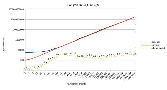
When sorting an int64, radix sort is “only” two to three times faster than std::sort. At least once you have more than 500 elements in your array. Since the difference in scale is linear though, we should be able to decrease the gap further by sorting bigger input data:

Aha, it looks like when we use sixteen bytes of data as the sort key, radix sort is finally slower than std::sort. At this point my implementation of radix sort has to do 18 passes over the input data, shuffling back and forth between the two buffers sixteen times. At some point that had to be slow. Note though that this does not mean that you can not sort large structs using radix sort. It only means that the sort key that you provide to radix sort has to be small. The size of the struct matters less. To prove that point here are the measurements for sorting a sixteen byte struct using an eight byte key:

When using a smaller key, radix sort is faster again. One thing to note though is that it’s not as fast as as when we were just sorting an int64. That suggests that maybe radix sort gets slower relative to std::sort as the size of the struct increases. The performance depends on the key size and the data size. So I decided to calculate the relative speed for a vector of size 2048. Meaning I did the above measurements with 2048 for “number of elements” and varied the key size and the data size, and plotted that in a table:

Time (in microseconds) to sort 2048 elements			key size
			1	4	16	64	256
data size	1	radix sort	16
		std::sort	81
		relative speed	5.2
	4	radix sort	18	24
		std::sort	88	87
		relative speed	4.8	3.7
	16	radix sort	24	40	123
		std::sort	100	97	112
		relative speed	4.1	2.4	0.9
	64	radix sort	57	119	347	1881
		std::sort	141	138	150	254
		relative speed	2.4	1.2	0.4	0.1
	256	radix sort	144	341	1195	5501	17657
		std::sort	413	443	459	577	698
		relative speed	2.9	1.3	0.4	0.1	0.04

One thing I should note is that my benchmark loop also generated 2048 random numbers. So the measurements above are really for generating 2048 random numbers using std::mt19937_64, and then sorting those random numbers. For the key size of 64 I had to generate eight random numbers and for the key size of 256 I had to generate 32 random numbers, so the overhead for the random number generation is larger in those columns.

So what can we read from this table? There are two main things to notice:

1. As the key size increases (reading from left to right), radix sort gets much slower. std::sort also slows down, but not by as much. When sorting one byte (two passes) radix sort is always faster. Same thing when sorting four bytes (five passes). At sixteen bytes (eighteen passes in my implementation, but you could do it in seventeen) radix sort starts to lose, especially when the data to move around is large. Moving the data back and forth sixteen times is just slow.
2. When the data size increases (reading from top to bottom) radix sort also gets slower relative to std::sort. However it looks like a data size increase does not cause radix sort to switch from being faster to being slower. In fact the gap in absolute terms actually widens every time that the data size increases.

The main reason why std::sort is not affected as much by an increase in key size is that it uses std::lexicographical_compare. Meaning if I have a key of size 256, which in my case was just a std::array<uint64_t, 32> and if the first entry in the key differs, then std::sort can early out and doesn’t even have to look at the remaining bytes. Since radix sort starts sorting at the least significant digit, it has to actually look at every single byte in the key. There is a variant of radix sort that looks at the most significant digit first, so it should perform better for larger keys, but I won’t talk about that too much in this piece.

All of this being said, how does radix sort perform on my initial use case of sorting a std::pair<bool, float>?

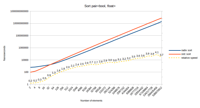
Radix sort performs very well on my initial use case. It’s faster starting at 64 elements in the array. That’s because this is the same speed as sorting by a four byte int, and then by a boolean. And sorting by a boolean is the fastest possible version of counting sort. You don’t even need the buffer of 256 counts, you only need to count how many “false” elements there are in the array. So adding a boolean to something will barely slow it down when using radix sort. Actually let’s talk about some more optimizations:

Performance Tricks

1. As just mentioned, you can write a faster version of counting sort for booleans. You don’t need to keep track of 256 counts for booleans, you just need one: How many “false” elements there were. Then you write all “true” elements starting at that offset, and all “false” elements starting at offset 0.
2. When sorting multiple bytes, you can combine the first two loops of all of them. For example when sorting four bytes, the straightforward implementation is to just call counting_sort four times. Then you would get eight passes over the input data. But if you allocate four counting buffers of size 256 on the stack, you can initialize all of them in one loop, and turn all of them into prefix sums in one loop. Then you only have to do five passes in total over the data.
3. The article that explains how to sort floating point numbers using radix sort also has a trick of sorting 11 bits at a time. Instead of sorting one byte at a time. The benefit of that is that you can sort a 32 bit number in four passes instead of five. I tried that, and for me it only gave me performance benefits if the input data is between 1024 and 4096 elements large. For any input sizes larger or smaller than that, sorting one byte at a time was faster. The reason for these numbers is that when sorting 11 bits, the counting array is of size 2048, and apparently if you do the math, the algorithm is fastest when the counting array is roughly the same size as the input data. I haven’t looked too much into that.
4. In my implementation of counting_sort above I use an array of type size_t[256]. If you know that each of the buckets in there is less than four billion elements in size, you could also use a uint32_t[256]. In fact I use a different type depending on the size of the input data. This does actually help because the main cost in counting_sort is cache misses. So if your count array is small, that means more of the other arrays can be in the cache.

Linear Time Sorting

Now that we know that radix sort can be fast, we can write a sorting algorithm that has O(n) for many inputs. I think that std::sort should be implemented like this:

template<typename It, typename OutIt, typename ExtractKey>
bool linear_sort(It begin, It end, OutIt buffer_begin, ExtractKey && key)
{
    std::ptrdiff_t num_elements = end - begin;
    auto compare_keys = [&](auto && lhs, auto && rhs)
    {
        return key(lhs) < key(rhs);
    };
    if (num_elements <= 16)
    {
        insertion_sort(begin, end, compare_keys);
        return false;
    }
    else if (num_elements <= 1024 || radix_sort_pass_count<ExtractKey, It>::value > 10)
    {
        std::sort(begin, end, compare_keys);
        return false;
    }
    else
        return radix_sort(begin, end, buffer_begin, std::forward<ExtractKey>(key));
}

First, the interface: Since this calls radix_sort, you have to provide a buffer that has the same size as the input array and a function to extract the sort key from the object. There could be a second version of this function with a default argument for the extract key function that just returns the value directly. So you sort can any type that radix sort supports. You would only have to provide an ExtractKey function for custom structs.

Next we decide which algorithm to use based on the number of elements. For a small number of elements, insertion_sort is generally thought to be the fastest algorithm. And for that I build a comparison function from the ExtractKey object. For a medium number of elements I would call std::sort. And for a large number of elements I would call radix_sort.

There is one more case where I call std::sort instead of radix_sort, and that is when radix sort would have to do a lot of passes over the input data. I can calculate how many passes radix sort has to do at compile time.

And finally the return value is a boolean that says whether the result was stored in the input buffer or in the output buffer. Depending on how many passes radix_sort has to do, the result could end up in either. So for example when sorting an int32, the function would return false because radix sort does four passes and the data ends up back in the input array, but when sorting a std::pair<bool, float> the function would return true because radix sort does five passes and the data ends up in the output array. The calling function then has to do something sensible with this information. If the two buffers are std::vectors, it could just swap them afterwards to get the data where it wants it to be.

Based on the benchmarks above, this algorithm would be several times faster than current implementations of std::sort for many inputs, and it would never be slower than std::sort.

How would we go about getting something like this into the standard? Well clearly we can’t change the interface of std::sort at this point. We could provide a function called std::sort_copy though that would have the above interface and could call radix_sort when that makes sense.

There is an in-place version of radix sort. If we used that, we could even use radix sort in std::sort. Except that we can’t get the ExtractKey function because std::sort takes a comparison functor. One solution for that would be to provide a customization point called std::sort_key which would work similar to std::hash. If your class provides a specialization for std::sort_key, std::sort is allowed to use an in-place version of radix sort when it makes sense, or it could build a comparison operator using std::sort_key and fall back to the old behavior.

In-place Radix Sort

This entire time we were building on top of counting_sort which needs to copy results to a different buffer. But if we could provide a version of radix sort that does all operations in one buffer, we could get that version into std::sort.

The in-place version of radix sort has one other very nice benefit: It starts sorting at the most significant digit. The version of radix sort that we used above started sorting at the least significant digit. This made radix sort slow for large keys because it always had to look at every byte of the key. The in-place version could early out after looking at the first byte, which would potentially make it much faster for large keys.

I will sketch out how in-place radix sort works, but I’ll leave the work of implementing it and measuring it to “future work.” I’ll explain why I didn’t implement it after I explain how it works.

We can’t build on top of counting sort because counting sort needs to copy results into a new buffer. But there is an in-place O(n) sorting algorithm called American Flag Sort. It works similar to counting sort in that you need an array to count how often each element appears. So if we sort bytes, we also need a count array of 256 elements. Then we also compute the prefix sum of this count array, like we did in counting sort. Only the final loop is different:

In the final loop of counting sort, we would directly move elements into the position that they need to be at. The prefix sum would tell us directly what the right position is. Since American Flag Sort is in-place, we need to swap instead. So let’s say the first element in the array actually wants to be at position 5. We swap it with whatever was at position 5. If the new element actually wants to be at position 3, we swap it with whatever was at position 3. We keep doing this until we find an element that actually wants to be the first element of the array. Only then do we move on to the second element in the array.

What tends to happen is that all the swapping at the first element moves a lot of elements into the right positions. Then all the swapping at the second element moves a lot more elements into the right position. So by the time that we’re a third of the way through the array, most elements are actually already sorted. So a lot of work happens on the first few elements, but at the later elements you mostly just determine that the elements are already where they want to be.

If you implement this you will need two copies of the prefix array. One copy that you change as you swap elements into place, (so that if two elements want to be in the bucket starting at position 5, the first one gets moved to position 5, and the second one to position 6) and one copy that you leave unchanged so that you can determine whether the element is already in the bucket that it wants to be in. (otherwise the element that you swapped into position 5 would think that its bucket now starts at position 6)

Now that we know how American Flag Sort works, we can implement radix sort on top of this. For that, American Flag Sort has to return the 256 offsets into the 256 buckets that it created. Then we call American Flag Sort again to sort within each of those 256 buckets, using the next byte in the key as the byte that we want to sort on. Meaning for a four byte integer, we have to sort recursively within a smaller bucket three more times after the initial sort. Since there’s 256 buckets and each of those gets split into 256 buckets after the second iteration and each of those gets split again after the third iteration, that means that we’ll call the function 256^3 times. Since that is a crazy number, we can just call insertion_sort for any bucket that is less than 16 elements in size, which will be most buckets. And actually since the in-place radix sort isn’t stable, we can also just call std::sort for any bucket that is less than 1024 elements in size. That gets the number of recursive calls down by a lot.

This sounds simple: Use American Flag Sort to subdivide into 256 buckets using the first byte, then sort each of those buckets recursively using the remaining bytes as sort key. The problem that I ran into was that I had generalized radix sort to work on std::pair, std::tuple and std::array. On the in-place version these were far more complicated because you have to pass the logic for advancing and the next comparison function through all recursion layers. Especially the std::tuple code drove me template-crazy. Since American Flag Sort was also significantly slower than counting sort, I abandoned the in-place version for now and decided to leave that for future work.

So for now the takeaway is this: There is an in-place version of radix sort, but for now I decided that it’s too much work to implement. The part that I did implement looked several times slower than the copying radix sort. It might still be faster than std::sort, but I haven’t measured that.

Why Radix Sort Isn’t Popular

In this article I found that radix sort is several times faster than std::sort for what seem like pretty normal use cases. So why isn’t it used all over the place? I did a quick poll at work, and many people had heard of it, but didn’t know how to use it or whether it was even worth using at all. Which is exactly what I was like before I started this investigation. So why isn’t it popular? I have a few explanations

1. Size overhead: Radix sort requires a second array of the same size to store the data in. If your data is small you may not want to pay for the overhead of allocating and freeing a second buffer. If your data is large you may not have enough memory to have that second buffer. Radix sort may still be a great option if your data is sized somewhere in the middle, but using radix sort means that you have to worry about these things.
2. Can’t use radix sort on variable sized keys. The version of radix sort presented here only works on fixed sized keys. So it can’t sort strings for example. The in-place version of radix sort can sort strings, but I didn’t look into that too much.
3. We used to always write custom comparison functions. If you don’t use std::make_tuple or std::tie to implement your comparison function, it may not be obvious how to use radix sort for your class. You need to know that you can sort tuples using radix sort, and you need to notice that you’re using tuples in your comparison functions already.
4. I can’t find any place that generalizes radix sort to std::pair, std::tuple and std::array. So this might actually be an original contribution of mine. Googling for it I can find mentions of using radix sort on tuples of ints, but it seems like those people don’t realize that you can generalize beyond that. Certainly nobody suggests that you could use radix sort on a std::pair<bool, float>. (for example the boost version of radix sort can not sort a std::pair<bool, float>, and boost code is usually way too generic) If you think that radix sort is only for integers, it’s not very useful.
5. Radix sort can not take advantage of already sorted data. It always has to do the same operations, no matter what the data looks like. std::sort can be much faster on already sorted data.

So there are certainly some good reasons for not using radix sort. There simply can’t be one best sorting algorithm. However I also think that radix sort lost some popularity due to historical accidents. People often don’t seem to think that it applies to their data even though it does.

Conclusion

Radix sort is an old algorithm, but I think it should be used more. Much more. Depending on what your sort key is, it will be several times faster than comparison based sorting algorithms.

Radix sort can be used to implement a general purpose O(n) sorting algorithm that automatically falls back to std::sort when that would be faster. I think the standard library should be modified so that it can provide this behavior. I think this is possible by offering an extension point called std::sort_key which would work similar to std::hash. Even without that the standard could provide std::sort_copy, which would promise O(n) sorting on small keys.

The final conclusion is that it’s worth learning something about algorithms even if you’ve programmed for a while. I learned how radix sort works because I’ve been watching an Introduction to Algorithms course by MIT. I didn’t expect to learn anything new in that course, but it’s already caused me to write this blog post, and it’s inspired me to take another stab at writing the worlds fastest hashtable. (in progress) So never stop learning, and try to fill in the gaps in your knowledge of the basics. You never know when it will be useful.

I have uploaded my implementation of radix sort here, licensed under the boost license.