I Wrote a Faster Sorting Algorithm
by Malte Skarupke
These days it’s a pretty bold claim if you say that you invented a sorting algorithm that’s 30% faster than state of the art. Unfortunately I have to make a far bolder claim: I wrote a sorting algorithm that’s twice as fast as std::sort for many inputs. And except when I specifically construct cases that hit my worst case, it is never slower than std::sort. (and even when I hit those worst cases, I detect them and automatically fall back to std::sort)
Why is that an unfortunate claim? Because I’ll probably have a hard time convincing you that I did speed up sorting by a factor of two. But this should turn out to be quite a lengthy blog post, and all the code is open source for you to try out on whatever your domain is. So I might either convince you with lots of arguments and measurements, or you can just try the algorithm yourself.
Following up from my last blog post, this is of course a version of radix sort. Meaning its complexity is lower than O(n log n). I made two contributions:
- I optimized the inner loop of in-place radix sort. I started off with the Wikipedia implementation of American Flag Sort and made some non-obvious improvements. This makes radix sort much faster than std::sort, even for a relatively small collections. (starting at 128 elements)
- I generalized in-place radix sort to work on arbitrary sized ints, floats, tuples, structs, vectors, arrays, strings etc. I can sort anything that is reachable with random access operators like operator[] or std::get. If you have custom structs, you just have to provide a function that can extract the key that you want to sort on. This is a trivial function which is less complicated than the comparison operator that you would have to write for std::sort.
If you just want to try the algorithm, jump ahead to the section “Source Code and Usage.”
O(n) Sorting
To start off with, I will explain how you can build a sorting algorithm that’s O(n). If you have read my last blog post, you can skip this section. If you haven’t, read on:
If you are like me a month ago, you knew for sure that it’s proven that the fastest possible sorting algorithm has to be O(n log n). There are mathematical proofs that you can’t make anything faster. I believed that until I watched this lecture from the “Introduction to Algorithms” class on MIT Open Course Ware. There the professor explains that sorting has to be O(n log n) when all you can do is compare items. But if you’re allowed to do more operations than just comparisons, you can make sorting algorithms faster.
I’ll show an example using the counting sort algorithm:
template<typename It, typename OutIt, typename ExtractKey>
void counting_sort(It begin, It end, OutIt out_begin, ExtractKey && extract_key)
{
    size_t counts[256] = {};
    for (It it = begin; it != end; ++it)
    {
        ++counts[extract_key(*it)];
    }
    size_t total = 0;
    for (size_t & count : counts)
    {
        size_t old_count = count;
        count = total;
        total += old_count;
    }
    for (; begin != end; ++begin)
    {
        std::uint8_t key = extract_key(*begin);
        out_begin[counts[key]++] = std::move(*begin);
    }
}
This version of the algorithm can only sort unsigned chars. Or rather it can only sort types that can provide a sort key that’s an unsigned char. Otherwise we would index out of range in the first loop. Let me explain how the algorithm works:
We have three arrays and three loops. We have the input array, the output array, and a counting array. In the first loop we fill the counting array by iterating over the input array, counting how often each element shows up.
The second loop turns the counting array into a prefix sum of the counts. So let’s say the array didn’t have 256 entries, but only 8 entries. And let’s say the numbers come up this often:
| index | 0 | 1 | 2 | 3 | 4 | 5 | 6 | 7 |
| count | 0 | 2 | 1 | 0 | 5 | 1 | 0 | 0 |
| prefix sum | 0 | 0 | 2 | 3 | 3 | 8 | 9 | 9 |
So in this case there were nine elements in total. The number 1 showed up twice, the number 2 showed up once, the number 4 showed up five times and the number 5 showed up once. So maybe the input sequence was { 4, 4, 2, 4, 1, 1, 4, 5, 4 }.
The final loop now goes over the initial array again and uses the key to look up into the prefix sum array. And lo and behold, that array tells us the final position where we need to store the integer. So when we iterate over that sequence, the 4 goes to position 3, because that’s the value that the prefix sum array tells us. We then increment the value in the array so that the next 4 goes to position 4. The number 2 will go to position 2, the next 4 goes to position 5 (because we incremented the value in the prefix sum array twice already) etc. I recommend that you walk through this once manually to get a feeling for it. The final result of this should be { 1, 1, 2, 4, 4, 4, 4, 4, 5 }.
And just like that we have a sorted array. The prefix sum told us where we have to store everything, and we were able to compute that in linear time.
Also notice how this works on any type, not just on integers. All you have to do is provide the extract_key() function for your type. In the last loop we move the type that you provided, not the key returned from that function. So this can be any custom struct. For example you could sort strings by length. Just use the size() function in extract_key, and clamp the length to at most 255. You could write a modified version of counting_sort that tells you where the position of the last partition is, so that you can then sort all long strings using std::sort. (which should be a small subset of all your strings so that the second pass on those strings should be fast)
In-Place Linear Time Sort
The above algorithm stores the sorted elements in a separate array. But it doesn’t take much to get an in-place sorting algorithm for unsigned chars: One thing we could try is that instead of moving the elements, we swap them.
The most obvious problem that we run into with that is that when we swap the first element out of the first spot, the new element probably doesn’t want to be in the first spot. It might want to be at position 10 instead. The solution for that is simple: Keep on swapping the first element until we find an element that actually wants to be in the first spot. Only when that has happened do we move on to the second item in the array.
The second problem that we then run into is that we’ll find a lot of partitions that are already sorted. We may not know however that those are already sorted. Imagine if we have the number 3 two times and it wants to be in positions six and seven. And lets say that as part of swapping the first element into place, we swap the first 3 to slot six, and the second 3 to slot seven. Now these are sorted and we don’t need to do anything with them any more. But when we advance on from the first element, we will at some point come across the 3 in slot six. And we’ll swap it to spot eight, because that’s the next spot that a 3 would go to. Then we find the next 3 and swap it to spot nine. Then we find the first 3 again and swap it to spot ten etc. This keeps going until we index out of bounds and crash.
The solution for the second problem is to keep a copy of the initial prefix array around so that we can tell when a partition is finished. Then we can skip over those partitions when advancing through the array.
With those two changes we have an in-place sorting algorithm that sorts unsigned chars. This is the American Flag Sort algorithm as described on Wikipedia.
In-Place Radix Sort
Radix sort takes the above algorithm, and generalizes it to integers that don’t fit into a single unsigned char. The in-place version actually uses a fairly simple trick: Sort one byte at a time. First sort on the highest byte. That will split the input into 256 partitions. Now recursively sort within each of those partitions using the next byte. Keep doing that until you run out of bytes.
If you do the math on that you will find that for a four byte integer you get 256^3 recursive calls: We subdivide into 256 partitions then recurse, subdivide each of those into 256 partitions and recurse again and then subdivide each of the smaller partitions into 256 partitions again and recurse a final time. If we actually did all of those recursions this would be a very slow algorithm. The way to get around that problem is to stop recursing when the number of items in a partition is less than some magic number, and to use std::sort within that sub-partition instead. In my case I stop recursing when a partition is less than 128 elements in size. When I have split an array into partitions that have less than that many elements, I call std::sort within these partitions.
If you’re curious: The reason why the threshold is at 128 is that I’m splitting the input into 256 partitions. If the number of partitions is k, then the complexity of sorting on a single byte is O(n+k). The point where radix sort gets faster than std::sort is when the loop that depends on n starts to dominate over the loop that depends on k. In my implementation that’s somewhere around 0.5k. It’s not easy to move it much lower than that. (I have some ideas, but nothing has worked yet)
Generalizing Radix Sort
It should be clear that the algorithm described in the last section works for unsigned integers of any size. But it also works for collections of unsigned integers, (including pairs and tuples) and strings. Just sort by the first element, then by the next, then by the next etc. until the partition sizes are small enough. (as a matter of fact the paper that Wikipedia names as the source for its American Flag Sort article intended the algorithm as a sorting algorithm for strings)
But it’s straightforward to generalize this to work on signed integers: Just shift all the values up into the range of the unsigned integer of the same size. Meaning for an int16_t, just cast to uint16_t and add 32768.
Michael Herf has also discovered a good way to generalize this to floating point numbers: Reinterpret cast the float to a uint32, then flip every bit if the float was negative, but flip only the sign bit if the float was positive. The same trick works for doubles and uint64s. Michael Herf explains why this works in the linked piece, but the short version of it is this: Positive floating point numbers already sort correctly if we just reinterpret cast them to a uint32. The exponent comes before the mantissa, so we would sort by the exponent first, then by the mantissa. Everything works out. Negative floating point numbers however would sort the wrong way. Flipping all the bits on them fixes that. The final remaining problem is that positive floating point numbers need to sort as bigger than negative numbers, and the easiest way to do that is to flip the sign bit since it’s the most significant bit.
Of the fundamental types that leaves only booleans and the various char types. Chars can just be reinterpret_casted to the unsigned types of the same size. Booleans could also be turned into a unsigned char, but we can also use a custom, more efficient algorithm for booleans: Just use std::partition instead of the normal sorting algorithm. And if we need to recurse because we’re sorting on more than one key, we can recurse into each of the partitions.
And just like that we have generalized in-place radix sort to all types. Now all it takes is a bunch of template magic to make the code do the right thing for each case. I’ll spare you the details of that. It wasn’t fun.
Optimizing the Inner Loop
The brief recap of the sorting algorithm for sorting one byte is:
- Count elements and build the prefix sum that tells us where to put the elements
- Swap the first element into place until we find an item that wants to be in the first position (according to the prefix sum)
- Repeat step 2 for all positions
I have implemented this sorting algorithm using Timo Bingmann’s Sound of Sorting. Here is a what it looks (and sounds) like:
As you can see from the video, the algorithm spends most of its time on the first couple elements. Sometimes the array is mostly sorted by the time that the algorithm advances forward from the first item. What you can’t see in the video is the prefix sum array that’s built on the side. Visualizing that would make the algorithm more understandable, (it would make clear how the algorithm can know the final position of elements to swap them directly there) but I haven’t done the work of visualizing that.
If we want to sort multiple bytes we recurse into each of the 256 partitions and do a sort within those using the next byte. But that’s not the slow part of this. The slow part is step 2 and step 3.
If you profile this you will find that this is spending all of its time on the swapping. At first I thought that that was because of cache misses. Usually when the line of assembly that’s taking a lot of time is dereferencing a pointer, that’s a cache miss. I’ll explain what the real problem was further down, but even though my intuition was wrong it drove me towards a good speed up: If we have a cache miss on the first element, why not try swapping the second element into place while waiting for the cache miss on the first one?
I already have to keep information about which elements are done swapping, so I can skip over those. So what I do is that I Iterate over all elements that have not yet been swapped into place, and I swap them into place. In one pass over the array, this will swap at least half of all elements into place. To see why, let’s think how this works in this list: { 4, 3, 1, 2 }: We look at the first element, the 4, and swap it with the 2 at the end, giving us this list: { 2, 3, 1, 4 }, then we look at the second element, the 3, and swap it with the 1, giving us this list: { 2, 1, 3, 4 } then we have iterated half-way through the list and find that all the remaining elements are sorted, (we do this by checking that the offset stored in the prefix sum array is the same as the initial offset of the next partition) so we’re done, but our list is not sorted. The solution for that is to say that when we get to the end of the list, we just start over from the beginning, swapping all unsorted elements into place. In that case we only need to swap the 2 into place to get { 1, 2, 3, 4 } at which point we know that all partitions are sorted and we can stop.
In Sound of Sorting that looks like this:
Implementation Details
This is what the above algorithm looks like in code:
struct PartitionInfo
{
    PartitionInfo()
        : count(0)
    {
    }

    union
    {
        size_t count;
        size_t offset;
    };
    size_t next_offset;
};

template<typename It, typename ExtractKey>
void ska_byte_sort(It begin, It end, ExtractKey & extract_key)
{
    PartitionInfo partitions[256];
    for (It it = begin; it != end; ++it)
    {
        ++partitions[extract_key(*it)].count;
    }
    uint8_t remaining_partitions[256];
    size_t total = 0;
    int num_partitions = 0;
    for (int i = 0; i < 256; ++i)
    {
        size_t count = partitions[i].count;
        if (count)
        {
            partitions[i].offset = total;
            total += count;
            remaining_partitions[num_partitions] = i;
            ++num_partitions;
        }
        partitions[i].next_offset = total;
    }
    for (uint8_t * last_remaining = remaining_partitions + num_partitions, * end_partition = remaining_partitions + 1; last_remaining > end_partition;)
    {
        last_remaining = custom_std_partition(remaining_partitions, last_remaining, [&](uint8_t partition)
        {
            size_t & begin_offset = partitions[partition].offset;
            size_t & end_offset = partitions[partition].next_offset;
            if (begin_offset == end_offset)
                return false;

            unroll_loop_four_times(begin + begin_offset, end_offset - begin_offset, [partitions = partitions, begin, &extract_key, sort_data](It it)
            {
                uint8_t this_partition = extract_key(*it);
                size_t offset = partitions[this_partition].offset++;
                std::iter_swap(it, begin + offset);
            });
            return begin_offset != end_offset;
        });
    }
}
The algorithm starts off similar to counting sort above: I count how many items fall into each partition. But I changed the second loop: In the second loop I build an array of indices into all the partitions that have at least one element in them. I need this because I need some way to keep track of all the partitions that have not been finished yet. Also I store the end index for each partition in the next_offset variable. That will allow me to check whether a partition is finished sorting.
The third loop is much more complicated than counting sort. It’s three nested loops, and only the outermost is a normal for loop:
The outer loop iterates over all of the remaining unsorted partitions. It stops when there is only one unsorted partition remaining. That last partition does not need to be sorted if all other partitions are already sorted. This is an important optimization because the case where all elements fall into only one partition is quite common: When sorting four byte integers, if all integers are small, then in the first call to this function, which sorts on the highest byte, all of the keys will have the same value and will fall into one partition. In that case this algorithm will immediately recurse to the next byte.
The middle loop uses std::partition to remove finished partitions from the list of remaining partitions. I use a custom version of std::partition because std::partition will unroll its internal loop, and I do not want that. I need the innermost loop to be unrolled instead. But the behavior of custom_std_partition is identical to that of std::partition. What this loop means is that if the items fall into partitions of different sizes, say for the input sequence { 3, 3, 3, 3, 2, 5, 1, 4, 5, 5, 3, 3, 5, 3, 3 } where the partitions for 3 and 5 are larger than the other partitions, this will very quickly finish the partitions for 1, 2 and 4, and then after that the outer loop and inner loop only have to iterate over the partitions for 3 and 5. You might think that I could use std::remove_if here instead of std::partition, but I need this to be non-destructive, because I will need the same list of partitions when making recursive calls. (not shown in this code listing)
The innermost loop finally swaps elements. It just iterates over all remaining unsorted elements in a partition and swaps them into their final position. This would be a normal for loop, except I need this loop unrolled to get fast speeds. So I wrote a function called “unroll_loop_four_times” that takes an iterator and a loop count and then unrolls the loop.
Why this is Faster
This new algorithm was immediately much faster than American Flag Sort. Which made sense because I thought I had tricked the cache misses. But as soon as I profiled this I noticed that this new sorting algorithm actually had slightly more cache misses. It also had more branch mispredictions. It also executed more instructions. But somehow it took less time. This was quite puzzling so I profiled it whichever way I could. For example I ran it in Valgrind to see what Valgrind thought should be happening. In Valgrind this new algorithm was actually slower than American Flag Sort. That makes sense: Valgrind is just a simulator, so something that executes more instructions, has slightly more cache misses and slightly more branch mispredictions would be slower. But why would it be faster running on real hardware?
It took me more than a day of staring at profiling numbers before I realized why this was faster: It has better instruction level parallelism. You couldn’t have invented this algorithm on old computers because it would have been slower on old computers. The big problem with American Flag Sort is that it has to wait for the current swap to finish before it can start on the next swap. It doesn’t matter that there is no cache-miss: Modern CPUs could execute several swaps at once if only they didn’t have to wait for the previous one to finish. Unrolling the inner loop also helps to ensure this. Modern CPUs are amazing, so they could actually run several loops in parallel even without loop unrolling, but the loop unrolling helps.
The Linux perf command has a metric called “instructions per cycle” which measures instruction level parallelism. In American Flag Sort my CPU achieves 1.61 instructions per cycle. In this new sorting algorithm it achieves 2.24 instructions per cycle. It doesn’t matter if you have to do a few instructions more, if you can do 40% more at a time.
And the thing about cache misses and branch mispredictions turned out to be a red herring: The numbers for those are actually very low for both algorithms. So the slight increase that I saw was a slight increase to a low number. Since there are only 256 possible insertion points, chances are that a good portion of them are always going to be in the cache. And for many real world inputs the number of possible insertion points will actually be much lower. For example when sorting strings, you usually get less than thirty because we simply don’t use that many different characters.
All that being said, for small collections American Flag Sort is faster. The instruction level parallelism really seems to kick in at collections of more than a thousand elements. So my final sort algorithm actually looks at the number of elements in the collection, and if it’s less than 128 I call std::sort, if it’s less than 1024 I call American Flag Sort, and if it’s more than that I run my new sorting algorithm.
std::sort is actually a similar combination, mixing quick sort, insertion sort and heap sort, so in a sense those are also part of my algorithm. If I tried hard enough, I could construct an input sequence that actually uses all of these sorting algorithms. That input sequence would be my very worst case: I would have to trigger the worst case behavior of radix sort so that my algorithm falls back to std::sort, and then I would also have to trigger the worst case behavior of quick sort so that std::sort falls back to heap sort. So let’s talk about worst cases and best cases.
Best Case and Worst Case
The best case for my implementation of radix sort is if the inputs fit in few partitions. For example if I have a thousand items and they all fall into only three partitions, (say I just have the number 1 a hundred times, the number 2 four hundred times, and the number 3 five hundred times) then my outer loops do very little and my inner loop can swap everything into place in nice long uninterrupted runs.
My other best case is on already sorted sequences: In that case I iterate over the data exactly twice, once to look at each item, and once to swap each item with itself.
The worst case for my implementation can only be reached when sorting variable sized data, like strings. For fixed size keys like integers or floats, I don’t think there is a really bad case for my algorithm. One way to construct the worst case is to sort the strings “a”, “ab”, “abc”, “abcd”, “abcde”, “abcdef” etc. Since radix sort looks at one byte at a time, and that byte only allows it to split off one item, this would take O(n^2) time. My implementation detects this by recording how many recursive calls there were. If there are too many, I fall back to std::sort. Depending on your implementation of quick sort, this could also be the worst case for quick sort, in which case std::sort falls back to heap sort. I debugged this briefly and it seemed like std::sort did not fall back to heap sort for my test case. The reason for that is that my test case was sorted data and std::sort seems to use the median-of-three rule for pivot selection, which selects a good pivot on already sorted sequences. Knowing that, it’s probably possible to create sequences that hit the worst case both for my algorithm and for the quick sort used in std::sort, in which case the algorithm would fall back to heap sort. But I haven’t attempted to construct such a sequence.
I don’t know how common this case is in the real world, but one trick I took from the boost implementation of radix sort is that I skip over common prefixes. So if you’re sorting log messages and you have a lot of messages that start with “warning:” or “error:” then my implementation of radix sort would first sort those into separate partitions, and then within each of those partitions it would skip over the common prefix and continue sorting at the first differing character. That behavior should help reduce how often we hit the worst case.
Currently I fall back to std::sort if my code has to recurse more than sixteen times. I picked that number because that was the first power of two for which the worst case detection did not trigger when sorting some log files on my computer.
Algorithm Summary and Naming
The sorting algorithm that I provide as a library is called “Ska Sort”. Because I’m not going to come up with new algorithms very often in my lifetime, so might as well put my name on one when I do. The improved algorithm for sorting bytes that I described above in the sections “Optimizing the Inner Loop” and “Implementation Details” is only a small part of that. That algorithm is called “Ska Byte Sort”.
In summary, Ska Sort:
- Is an in-place radix sort algorithm
- Sorts one byte at a time (into 256 partitions)
- Falls back to std::sort if a collection contains less than some threshold of items (currently 128)
- Uses the inner loop of American Flag Sort if a collection contains less than a larger threshold of items (currently 1024)
- Uses Ska Byte Sort if the collection is larger than that
- Calls itself recursively on each of the 256 partitions using the next byte as the sort key
- Falls back to std::sort if it recurses too many times (currently 16 times)
- Uses std::partition to sort booleans
- Automatically converts signed integers, floats and char types to the correct unsigned integer type
- Automatically deals with pairs, tuples, strings, vectors and arrays by sorting one element at a time
- Skips over common prefixes of collections. (for example when sorting strings)
- Provides two customization points to extract the sort key from an object: A function object that can be passed to the algorithm, or a function called to_radix_sort_key() that can be placed in the namespace of your type
So Ska Sort is a complicated algorithm. Certainly more complicated than a simple quick sort. One of the reasons for this is that in Ska Sort, I have a lot more information about the types that I’m sorting. In comparison based sorting algorithms all I have is a comparison function that returns a bool. In Ska Sort I can know that “for this collection, I first have to sort on a boolean, then on a float” and I can write custom code for both of those cases. In fact I often need custom code: The code that sorts tuples has to be different from the code that sorts strings. Sure, they have the same inner loop, but they both need to do different work to get to that inner loop. In comparison based sorting you get the same code for all types.
Optimizations I Didn’t Do
If you’ve got enough time on your hands that you clicked on the pieces I linked above, you will find that there are two optimizations that are considered important in my sources that I didn’t do.
The first is that the piece that talks about sorting floating point numbers sorts 11 bits at a time, instead of one byte at a time. Meaning it subdivides the range into 2048 partitions instead of 256 partitions. The benefit of this is that you can sort a four byte integer (or a four byte float) in three passes instead of four passes. I tried this in my last blog post and found it to only be faster for a few cases. In most cases it was slower than sorting one byte at a time. It’s probably worth trying that trick again for in-place radix sort, but I didn’t do that.
The second is that the American Flag Sort paper talks about managing recursions manually. Instead of making recursive calls, they keep a stack of all the partitions that still need to be sorted. Then they loop until that stack is empty. I didn’t attempt this optimization because my code is already far too complex. This optimization is easier to do when you only have to sort strings because you always use the same function to extract the current byte. But if you can sort ints, floats, tuples, vectors, strings and more, this is complicated.
Performance
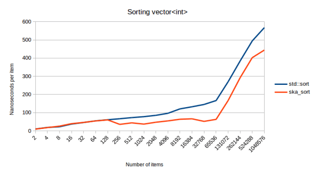
Finally we get to how fast this algorithm actually is. Since my last blog post I’ve changed how I calculate these numbers. In my last blog post I actually made a big mistake: I measured how long it takes to set up my test data and to then sort it. The problem with that is that the set up can actually be a significant portion of the time. So this time I also measure the set up separately and subtract that time from the measurements so that I’m left with only the time it takes to actually sort the data. With that let’s get to our first measurement: Sorting integers: (generated using std::uniform_int_distribution)

This graph shows how long it takes to sort various numbers of items. I didn’t mention ska_sort_copy before, but it’s essentially the algorithm from my last blog post, except that I changed it so that it falls back to ska_sort instead of falling back to std::sort. (ska_sort may still decide to fall back to std::sort of course)
One problem I have with this graph that even though I made the scale logarithmic, it’s still very difficult to see what’s going on. Last time I added another line at the bottom that showed the relative scale, but this time I have a better approach. Instead of a logarithmic scale, I can divide the total time by the number of items, so that I get the time that the sort algorithm spends per item:

With this visualization, we can see much more clearly what’s going on. All pictures below use “nanoseconds per item” as scale, like in this graph. Let’s analyze this graph a little:
For the first couple items we see that the lines are essentially the same. That’s because for less than 128 elements, I fall back to std::sort. So you would expect all of the lines to be exactly the same. Any difference in that area is measurement noise.
Then past that we see that std::sort is exactly a O(n log n) sorting algorithm. It goes up linearly when we divide the time by the number of items, which is exactly what you’d expect for O(n log n). It’s actually impressive how it forms an exactly straight line once we’re past a small number of items. ska_sort_copy is truly an O(n) sorting algorithm: The cost per item stays mostly constant as the total number of items increases. But ska_sort is… more complicated.
Those waves that we’re seeing in the ska_sort line have to do with the number of recursive calls: ska_sort is fastest when the number of items is large. That’s why the line starts off as decreasing. But then at some point we have to recurse into a bunch of partitions that are just over 128 items in size, which is slow. Then those partitions grow as the number of items increase and the algorithm is faster again, until we get to a point where the partitions are over 128 elements in size again, and we need to add another recursive step. One way to visualize this is to look at the graph of sorting a collection of int8_t:
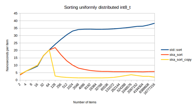
As you can see the cost per item goes down dramatically at the beginning. Every time that the algorithm has to recurse into other partitions, we see that initial part of the curve overlaid, giving us the waves of the graph for sorting ints.
One point I made above is that ska_sort is fastest when there are few partitions to sort elements into. So let’s see what happens when we use a std::geometric_distribution instead of a std::uniform_int_distribution:

This graph is sorting four byte ints again, so you would expect to see the same “waves” that we saw in the uniformly distributed ints. I’m using a std::geometric_distribution with 0.001 as the constructor argument. Which means it generates numbers from 0 to roughly 18000, but most numbers will be close to zero. (in theory it can generate numbers that are much bigger, but 18882 is the biggest number I measured when generating the above data) And since most numbers are close to zero, we will see few recursions and because of that we see few waves, making this many times faster than std::sort.
Btw that bump at the beginning is surprising to me. For all other data that I could find, ska_sort starts to beat std::sort at 128 items. Here it seems like ska_sort only starts to win later. I don’t know why that is. I might investigate it at a different point, but I don’t want to change the threshold because this is a good number for all other data. Changing the threshold would move all other lines up by a little. Also since we’re sorting few items there, the difference in absolute terms is not that big: 15.8 microseconds to 16.7 microseconds for 128 items, and 32.3 microseconds to 32.9 microseconds for 256 items.
Let’s look at some more use cases. Here is my “real world” use case that I talked about in the last blog post, where I had to sort enemies in a game by distance to the player. But I wanted all enemies that are currently in combat to come first, sorted by distance, followed by all enemies that are not in combat, also sorted by distance. So I sort by a std::pair:

This turned out to be the same graph as sorting ints, except every line is shifted up by a bit. Which I guess I should have expected. But it’s good to see that the conversion trick that I have to do for floats and the splitting I have to do for pairs does not add significant overhead. A more interesting graph is the one for sorting int64s:
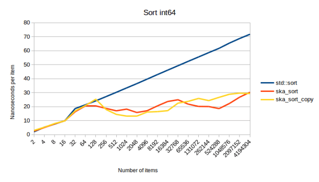
This is the point where ska_sort_copy is sometimes slower than ska_sort. I actually decided to lower the threshold where ska_sort_copy falls back to ska_sort: It will now only do the copying radix sort when it has to do less than eight iterations over the input data. Meaning I have changed the code, so that for int64s ska_sort_copy actually just calls ska_sort. Based on the above graph you might argue that it should still do the copying radix sort, but here is a measurement of sorting an 128 byte struct that has an int64 as a sort key:
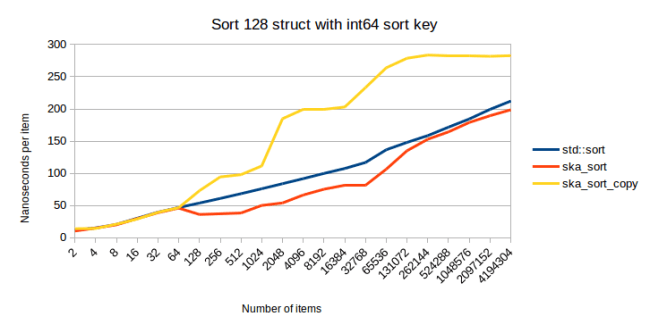
As the structs get larger, ska_sort_copy gets slower. Because of this I decided to make ska_sort_copy fall back to ska_sort for sort keys of this size.
One other thing to notice from the above graph is that it looks like std::sort and ska_sort get closer. So does ska_sort ever become slower? It doesn’t look like it. Here’s what it looks like when I sort a 1024 byte struct:
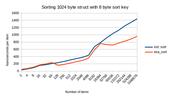
Once again this is a very interesting graph. I wish I could spend time on investigating where that large gap at the end comes from. It’s not measurement noise. It’s reproducible. The way I build these graphs is that I run Google Benchmark thirty times to reduce the chance of random variation.
Talking about large data, in my last blog post my worst case was sorting a struct that has a 256 byte sort key. Which in this case means using a std::array as a sort key. This was very slow on copying radix sort because we actually have to do 256 passes over the data. In-place radix sort only has to look at enough bytes until it’s able to tell two pieces of data apart, so it might be faster. And looking at benchmarks, it seems like it is:

ska_sort_copy will fall back to ska_sort for this input, so its graph will look identical. So I fixed the worst case from my last blog post. One thing that I couldn’t profile in my last blog post was sorting of strings, because ska_sort_copy simply can not sort strings because it can not sort variable sized data.
So let’s look at what happens when I’m sorting strings:

The way I build the input data here is that I take between one and three random words from my words file and concatenate them. Once again I am very happy to see how well my algorithm does. But this was to be expected: It was already known that radix sort is great for sorting strings.
But sorting strings is also when I can hit my worst case. In theory you might get cases where you have to do many passes over the data, because there simply are a lot of bytes in the input data and a lot of them are similar. So I tried what happens when I sort strings of different length, concatenating between zero and ten words from my words file:

What we see here is that ska_sort seems to become a O(n log n) algorithm when sorting millions of long strings. However it doesn’t get slower than std::sort. My best guess for the curve going up like that is that ska_sort has to do a lot of recursions on this data. It doesn’t do enough recursions to trigger my worst case detection, but those recursions are still expensive because they require one more pass over the data.
One thing I tried was lowering my recursion limit to eight, in which case I do hit my worst case detection starting at a million items. But the graph looks essentially unchanged in that case. The reason is that it’s a false positive: I didn’t actually hit my worst case. The sorting algorithm still succeeded at splitting the data into many smaller partitions, so when I fall back to std::sort, it has a much easier time than it would have had sorting the whole range.
Finally, here is what it looks like when I sort containers that are slightly more complicated than strings:
For this I generate vectors with between 0 and 20 ints in them. So I’m sorting a vector of vectors. That spike at the end is very interesting. My detection for too many recursive calls does not trigger here, so I’m not sure why sorting gets so much more expensive. Maybe my CPU just doesn’t like dealing with this much data. But I’m happy to report that ska_sort is faster than std::sort throughout, like in all other graphs.
Since ska_sort seems to always be faster, I also generated input data that intentionally triggers the worst case for ska_sort. The below graph hits the worst case immediately starting at 128 elements. But ska_sort detects that and falls back to std::sort:

For this I’m sorting random combinations of the vectors {}, { 0 }, { 0, 1 }, { 0, 1, 2 }, … { 0, 1, 2, … , 126, 127 }. Since each element only tells my algorithm how to split off 1/128th of the input data, it would have to recurse 128 times. But at the sixteenth recursion ska_sort gives up and falls back to std::sort. In the above graph you see how much overhead that is. The overhead is bigger than I like, especially for large collections, but for smaller collections it seems to be very low. I’m not happy that this overhead exists, but I’m happy that ska_sort detects the worst case and at least doesn’t go O(n^2).
Problems
Ska_sort isn’t perfect and it has problems. I do believe that it will be faster than std::sort for nearly all data, and it should almost always be preferred over std::sort.
The biggest problem it has is the complexity of the code. Especially the template magic to recursively sort on consecutive bytes. So for example currently when sorting on a std::pair<int, int> this will instantiate the sorting algorithm eight times, because there will be eight different functions for extracting a byte out of this data. I can think of ways to reduce that number, but they might be associated with runtime overhead. This needs more investigation, but the complexity of the code is also making these kinds of changes difficult. For now you can get slow compile times with this if your sort key is complex. The easiest way to get around that is to try to use a simpler sort key.
Another problem is that I’m not sure what to do for data that I can’t sort. For example this algorithm can not sort a vector of std::sets. The reason is that std::set does not have random access operators, and I need random access when sorting on one element at a time. I could write code that allows me to sort std::sets by using std::advance on iterators, but it might be slow. Alternatively I could also fall back to std::sort. Right now I do neither: I simply give a compiler error. The reason for that is that I provide a customization point, a function called to_radix_sort_key(), that allows you to write custom code to turn your structs into sortable data. If I did an automatic fallback whenever I can’t sort something, using that customization point would be more annoying: Right now you get an error message when you need to provide it, and when you have provided it, the error goes away. If I fall back to std::sort for data that I can’t sort, your only feedback for would be that sorting is slightly slower. You would have to either profile this and compare it to std::sort, or you would have to step through the sorting function to be sure that it actually uses your implementation of to_radix_sort_key(). So for now I decided on giving an error message when I can’t sort a type. And then you can decide whether you want to implement to_radix_sort_key() or whether you want to use std::sort.
Another problem is that right now there can only be one sorting behavior per type. You have to provide me with a sort key, and if you provide me with an integer, I will sort your data in increasing order. If you wanted it in decreasing order, there is currently no easy interface to do that. For integers you could solve this by flipping the sign in your key function, so this might not be too bad. But it gets more difficult for strings: If you provide me a string then I will sort the string, case sensitive, in increasing order. There is currently no way to do a case-insensitive sort for strings. (or maybe you want number aware sorting so that “bar100” comes after “bar99”, also can’t do that right now) I think this is a solvable problem, I just haven’t done the work yet. Since the interface of this sorting algorithm works differently from existing sorting algorithms, I have to invent new customization points.
Source Code and Usage
I have uploaded the code for this to github. It’s licensed under the boost license.
The interface works slightly differently from other sorting algorithms. Instead of providing a comparison function, you provide a function which returns the sort key that the sorting algorithm uses to sort your data. For example let’s say you have a vector of enemies, and you want to sort them by distance to the player. But you want all enemies that are in combat with the player to come first, sorted by distance, and then all enemies that are not in combat, also sorted by distance. The way to do that in a classic sorting algorithm would be like this:
std::sort(enemies.begin(), enemies.end(), [](const Enemy & lhs, const Enemy & rhs)
{
    return std::make_tuple(!is_in_combat(lhs), distance_to_player(lhs))
         < std::make_tuple(!is_in_combat(rhs), distance_to_player(rhs));
});
In ska_sort, you would do this instead:
ska_sort(enemies.begin(), enemies.end(), [](const Enemey & enemy)
{
    return std::make_tuple(!is_in_combat(enemy), distance_to_player(enemy));
});
As you can see the transformation is fairly straightforward. Similarly let’s say you have a bunch of people and you want to sort them by last name, then first name. You could do this:
ska_sort(contacts.begin(), contacts.end(), [](const Contact & c)
{
    return std::tie(c.last_name, c.first_name);
});
It is important that I use std::tie here, because presumably last_name and first_name are strings, and you don’t want to copy those. std::tie will capture them by reference.
Oh and of course if you just have a vector of simple types, you can just sort them directly:
ska_sort(durations.begin(), durations.end());
In this I assume that “durations” is a vector of doubles, and you might want to sort them to find the median, 90th percentile, 99th percentile etc. Since ska_sort can already sort doubles, no custom code is required.
There is one final case and that is when sorting a collection of custom types. ska_sort only takes a single customization function, but what do you do if you have a custom type that’s nested? In that case my algorithm would have to recurse into the top-level-type and would then come across a type that it doesn’t understand. When this happens you will get an error message about a missing overload for to_radix_sort_key(). What you have to do is provide an implementation of the function to_radix_sort_key() that can be found using ADL for your custom type:
struct CustomInt
{
    int i;
};
int to_radix_sort_key(const CustomInt & i)
{
    return i.i;
}

//... later somewhere

std::vector<std::vector<CustomInt>> collections = ...;
ska_sort(collections.begin(), collections.end());
In this case ska_sort will call to_radix_sort_key() for the nested CustomInts. You have to do this because there is no efficient way to provide a custom extract_key function at the top level. (at the top level you would have to convert the std::vector<CustomInt> to a std::vector<int>, and that requires a copy)
Finally I also provide a copying sort function, ska_sort_copy, which will be much faster for small keys. To use it you need to provide a second buffer that’s the same size as the input buffer. Then the return value of the function will tell you whether the final sorted sequence is in the second buffer (the function returns true) or in the first buffer (the function return false).
std::vector<int> temp_buffer(to_sort.size());
if (ska_sort_copy(to_sort.begin(), to_sort.end(), temp_buffer.begin()))
    to_sort.swap(temp_buffer);
In this code I allocate a temp buffer, and if the function tells me that the result ended up in the temp buffer, I swap it with the input buffer. Depending on your use case you might not have to do a swap. And to make this fast you wouldn’t want to allocate a temp buffer just for the sorting. You’d want to re-use that buffer.
FAQ
I’ve talked to a few people about this, and the usual questions I get are all related to people not believing that this is actually faster.
Q: Isn’t Radix Sort O(n+m) where m is large so that it’s actually slower than a O(n log n) algorithm? (or alternatively: Isn’t radix sort O(n*m) where m is larger than log n?)
A: Yes, radix sort has large constant factors, but in my benchmarks it starts to beat std::sort at 128 elements. And if you have a large collection, say a thousand elements, radix sort is a very clear winner.
Q: Doesn’t Radix Sort degrade to a O(n log n) algorithm? (or alternatively: Isn’t the worst case of Radix Sort O(n log n) or maybe even O(n^2)?)
A: In a sense Radix Sort has to do log(n) passes over the data. When sorting an int16, you have to do two passes over the data. When sorting an int32, you have to do four passes over the data. When sorting an int64 you have to do eight passes etc. However this is not O(n log n) because this is a constant factor that’s independent of the number of elements. If I sort a thousand int32s, I have to do four passes over that data. If I sort a million int32s, I still have to do four passes over that data. The amount of work grows linearly. And if the ints are all different in the first byte, I don’t even have to do the second, third or fourth pass. I only have to do enough passes until I can tell them all apart.
So the worst case for radix sort is O(n*b) where b is the number of bytes that I have to read until I can tell all the elements apart. If you make me sort a lot of long strings, then the number of bytes can be quite large and radix sort may be slow. That is the “worst case” graph above. If you have data where radix sort is slower than std::sort (something that I couldn’t find except when intentionally creating bad data) please let me know. I would be interested to see if we can find some optimizations for those cases. When I tried to build more plausible strings, ska_sort was always clearly faster.
And if you’re sorting something fixed size, like floats, then there simply is no accidental worst case. You are limited by the number of bytes and you will do at most four passes over the data.
Q: If those performance graphs were true, we’d be radix sorting everything.
A: They are true. Not sure what to tell you. The code is on github, so try it for yourself. And yes, I do expect that we will be radix sorting everything. I honestly don’t know why everybody settled on Quick Sort back in the day.
Future Work
There are a couple obvious improvements that I may make to the algorithm. The algorithm is currently in a good state, but if I ever feel like working on this again, here are three things that I might do:
As I said in the problems section, there is currently no way to sort strings case-insensitive. Adding that specific feature is not too difficult, but you’d want some kind of generic way to customize sorting behavior. Currently all you can do is provide a custom sort key. But you can not change how the algorithm uses that sort key. You always get items sorted in increasing order by looking at one byte at a time.
When I fall back to std::sort, I re-start sorting from the beginning. As I said above I fall back to std::sort when I have split the input into partitions of less than 128 items. But let’s say that one of those partitions is all the strings starting with “warning:” and one partition is all the strings starting with “error:” then when I fall back to std::sort, I could skip the common prefix. I have the information of how many bytes are already sorted. I suspect that the fact that std::sort has to start over from the beginning is the reason why the lines in the graph for sorting strings are so parallel between ska_sort and std::sort. Making this optimization might make the std::sort fallback much faster.
I might also want to write a function that can either take a comparison function, or an extract_key function. The way it would work is that if you pass a function object that takes two arguments, this uses comparison based sorting, and if you pass a function object that takes one argument, this uses radix sorting. The reason for creating a function like that is that it could be backwards compatible to std::sort.
Summary
In Summary I have a sorting algorithm that’s faster than std::sort for most inputs. The sorting algorithm is on github and is licensed under the boost license, so give it a try.
I mainly did two things:
- I optimized the inner loop of in-place radix sort, resulting in the ska_byte_sort algorithm
- I provide an algorithm, ska_sort, that can perform Radix Sort on arbitrary types or combinations of types
To use it on custom types you need to provide a function that provides a “sort key” to ska_sort, which should be a int, float, bool, vector, string, or a tuple or pair consisting of one of these. The list of supported types is long: Any primitive type will work or anything with operator[], so std::array and std::deque and others will also work.
If sorting of data is critical to your performance (good chance that it is, considering how important sorting is for several other algorithms) you should try this algorithm. It’s fastest when sorting a large number of elements, but even for small collections it’s never slower than std::sort. (because it uses std::sort when the collection is too small)
The main lessons to learn from this are that even “solved” problems like sorting are worth revisiting every once in a while. And it’s always good to learn the basics properly. I didn’t expect to learn anything from an “Introduction to Algorithms” course but I already wrote this algorithm and I’m also tempted to attempt once again to write a faster hashtable.
If you do use this algorithm in your code, let me know how it goes for you. Thanks!

you dont have to convince me of anything– just tell me why people wont slowly adopt your algorithm if its twice as fast. i dont say that out of skepticism, just practicality. also if you did write the next generation of sort algorithm, i definitely want to brag that i knew you before you were famous. you can do the same if my programming language ever gets anywhere. ha! (no really, you can. if that ever happens. feel free to quote me.)
i met buzz aldrin once, and i might have the autograph of the guy that invented ethernet laying around, so if i meet the person that invented the next amazing sort algorithm, thats good stuff– i sincerely wish you luck with it. im already following your blog, so hopefully there will be more about this.
Please go back and understand that Big O notation is about worst case, not typical case. If your algorithm falls back to std::sort, it’s Big O notation is necessarily no better than std::sort.
I actually didn’t want to say what my final thoughts on the Big O complexity of ska_sort are, because it’s complicated. But I guess I use Big O notation all over the blog post, so I should have probably given a final “this is what the Big O complexity is.”
I know that counting_sort is O(n), but ska_sort is not. You can see that from several of the graphs. The part about O(n) sorting is just an introduction to convince you that you can sort things faster than O(n log n). Also you need to know counting sort to get to American Flag Sort, and you need that to get to ska_byte_sort.
Also I was able to create an input sequence where ska_sort is O(n^2). So we could stop there and say that ska_sort is O(n^2). Except that the complexity depends on the type that you’re sorting.
When sorting ints it’s not possible to create an input sequence that would result in O(n^2) complexity.
I do think that it’s less than O(n log n). The reason is that I only fall back to std::sort for partitions of less than 128 elements. So maybe it’s O(n log 128) which would just be O(n). But that’s not right.
I think the best clue is in how I created the worst case: I made it so that the algorithm had to look at a lot of bytes before it can tell the elements apart. To tell n elements apart in my worst case scenario it had to look at n bytes. So my best guess for the Big O complexity of this algorithm is O(n * b) where b is the number of bytes that the algorithm has to look at in order to tell elements apart. (or actually until it can tell elements apart enough that it can group them into partitions of 128 elements or fewer)
Which actually also has to be considered when looking at the the complexity of std::sort when sorting strings: It’s O(n * b * log n). A core assumption of the O(n log n) complexity of std::sort is that comparisons are constant time. But when sorting strings, comparisons can take hugely different amount of times.
One key difference of ska_sort compared to std::sort is that this b number shows up even when sorting small keys like ints: In std::sort the comparison is constant time for that. In ska_sort even for ints it has to do between one and four passes.
Big O notation is about “worst case” scenarios, but for given inputs. Quicksort, for example, has a well-known “pathological” behavior which is O(n^2) but only for specific inputs. We typically refer to it as being O(n log n) because that’s the “worst case” asymptotic behavior of the common inputs. We don’t call Quicksort O(n^2) even though that is it’s “worst case” input. For almost all common inputs, Quicksort is O(n log n). That’s how we usually talk about it.
If Ska sort is O(n)ish for most cases except for well-understood pathological cases, we can call it O(n)ish and make note that things can get much worse than that sometimes for specific inputs. std::sort is already a hybrid sort making use of Quicksort and Heapsort, and falling back to Insertion Sort for short runs. (the C stdlib sort routine is nearly the same but falls back to bubble sort in some implementations, if I remember correctly). If Insertion Sort is O(n^2) or if Quicksort’s worst case is known to be O(n^2) we could declare std::sort to be O(n^2), but when you look at actual graphs of performance on actual data you see that it’s asymptotically O(n log n).
What really matters in a sorting algorithm is the asymptotic performance of the algorithm over a range of real-world inputs. This is why the Python folks have had such lasting success with their “Timsort” algorithm, which seems to do much better than O(n log n) for many real-world data scenarios, even though it’s a hybrid of merge and insertion sorts which both should be O(n log n) or worse, especially in pathological cases.
If I can plug this algorithm into my software and achieve performance improvements for nearly all cases, and get a guarantee that it won’t be any worse than std::sort for the remainder, that’s a significant achievement that is worth significant attention.
Big O notation is not about worst case; Big O is about up-bounding the growth rate of a function. You can talk about Big O in context of best-case, worst-case, and average-cases, though often only the latter two are of much practical value.
You are comparing apples with oranges. std::sort just compares keys, you are using their values. There is a lot of theory on taking advantage on the value of the key (all the O(n) algorithms) and you are not comparing the speed of your algorithm with them. In most of the interesting cases you have to sort objects that you can just compare: you can do a.compare(b) that returns -1, 0, 1 and you have to sort only depending on that result.
I’m comparing sorting algorithms to sorting algorithms. I don’t think that’s apples to oranges. Why does it matter how the algorithm works internally? But I would gladly compare this against other radix sorts if you can show me any. I don’t think anyone has done the work of writing a general purpose radix sort like I have.
At least that is one of the two contributions that I claim to have made in this blog post.
Your algorithm can not be general, like std::sort.
How can you implement your algorithm when an array of comparable objects are given?
public void sort(Comparable v[]){
//write your code here
}
There’s a huge difference between key-based sorting and comparison-based sorting. Most of the time you don’t have access to internal fields of an object and only a comparison function is given. And this is useful in order to abstract.
It’s like comparing find_on_sorted_array(int elem, int v[]) that has O(log n) complexity (binary search) and find_on_array(int elem, int v[]) that has O(n) complexity (scan and compare). Of course with more assumptions you can obtain faster algorithms.
In the case of sorting, there is for example Timsort, that performs better than std::sort in real world data, because it assumes that real world data has some subparts that are already ordered, but if you randomly shuffle an array you won’t find any performance difference on sorting it.
By the way you should compare to some other algorithms of this kind, e.g. boost spreadsort.
My algorithm is general. It’s true that my algorithm can not sort everything that std::sort can sort, but that doesn’t mean it’s not general. std::sort can’t sort everything either.
So std::sort can sort a subset of all possible collections. My algorithm can sort a subset of that. Your argument says that the threshold for a “general” sorting algorithm is somewhere between the collections that I can sort and the collections that std::sort can sort. What if I wrote a sorting algorithm that can sort more than std::sort can sort? For example I could write one that doesn’t require random access iterators. Is std::sort no longer a “general” sorting algorithm as soon as I write that? Because it can’t sort everything that other sorting algorithms can sort?
The question is not whether the algorithm can sort everything, but whether it can sort useful collections. My algorithm can sort pretty much everything, especially since you can provide a custom key.
Or looking at it from a more practical point of view: The question isn’t whether it can sort everything, but whether it can sort your use case. The answer is: very most likely yes. If you have a real use case that this can not sort, I would actually be curious to know what that is. My contribution is that I wrote a radix sort that can sort pretty much everything. As far as I can tell that hasn’t been done before.
You do make a good point in that I should have probably compared this against boost spreadsort. Even though spreadsort can only sort very few types, it would still be useful to see whether I missed any optimizations that boost did.
I’m still not sure I understand, but well done!
Any part in particular that I should explain better? I might have kept things a bit too short in some of the sections, but this blog post was already very long.
Yes it was incredibly long (did you consider breaking up into a post series?). I think it was the “why it was faster” as you explain it’s not faster per-core, it just makes good use of the compiler ILP through it’s structure. I also didn’t understand why you thought it would get less cache misses or more implementation details of the process of profiling but I’m not sure I have to understand fully to appreciate.
https://en.wikipedia.org/wiki/Radix_sort
Please check the “Recursive forward radix sort example” section which describes exactly what you have implemented. The example presented there uses only 10 buckets for readability but the last phrase mentions that bytes make more sense (1 byte – 256 buckets, 2 – 65536 buckets, etc – depending on available memory and data set characteristics).
Not sure what your comment is. Isn’t that what I’m explaining in the section “In-Place Radix Sort”?
He’s basically saying “you haven’t invented a faster sort algorithm, you’ve just implemented an already known one”…I guess the overall take home here is “std::sort isn’t optimized for numerics!” and “if you use a different sort, optimized for them, and aren’t afraid to use a little more space [double?] during sorting, you can get a nice speedup!” (it might hit caches better than quicksort, and, as this paper said, use pipelining more efficiently) which is…interesting, at least to those of us hitherto unfamiliar with Radix sort. Maybe should be titled “guess, what, there’s an under appreciated sorting algorithm, which is faster than std::sort” , so thanks for the info! I found it’s even faster, in java, to use it than to use java’s built-in Arrays.sort(int[]). https://erik.gorset.no/2011/04/radix-sort-is-faster-than-quicksort.html Mind blown…
But that’s not what I’m claiming. I don’t claim to have invented radix sort. I claim to have made two improvements to radix sort. I made it faster and more general. I say that in the introduction.
Fair enough. Implementation details (like when is the “sweet spot” to convert to american flag sort, and the fact it can be used with tuples, etc.) are fun! 🙂
Very interesting. Is the large variation in part due to std::sort being not particularly great? I would be very surprised if large corporate applications like oracle databases didn’t use a similar idea, which is to attempt to analyse the nature of the data and use difference methods accordingly.
Do you mean the variation within a graph or between graphs? Meaning “why is the sorting so much faster when sorting fewer elements than when sorting many elements?” or “why is the sorting so much faster when sorting one type than when sorting another type?”
In either case I didn’t look enough into the variations. I looked into some of the variation in a comment on my other blog post on radix sort, ( https://probablydance.com/2016/12/02/investigating-radix-sort/ ) and based on that I think this is mostly due to hardware artifacts. Meaning the curve goes up by a lot when the data goes from fitting into L2 cache to fitting into L3 cache. And then it goes up a lot again when it doesn’t fit into L3 cache any more.
The curve of std::sort is actually impressively stable. I think that’s because quick sort is ideal for the prefetcher of a CPU, so your data will usually be in the cache. ska_sort does a lot more “random” movements.
And yes, I would expect that they use radix sort in databases. In fact the lecture that I linked to as my inspiration for wanting to write a radix sort specifically talks about an example of using this to sort tables.
It used to be that radix sort was used whenever you have simple types. (which you do have in databases) One of my contributions is that I have generalized radix sort so that it works on nearly every type.
Wow reading my comment again I really failed to accurately get across what I meant O_o, apologies. I learnt more from your reply than I expected though!
What I meant originally was actually quite dreary in comparison, which was seeing that ska_sort has a large improvement over std::sort in many cases, do you think part of reason this improvement (which I called variation) was so large in some cases (as you say yourself, as large as 30%), is because std::sort is *already* bad/inefficient in comparison to the methods used in large data keeping systems and the like?
You should publish a paper on this.
Hmm maybe. I hadn’t thought of it. I didn’t really invent anything new. I guess I could write one paper about my optimization for the inner loop, and then I could write a second paper about how I combined several different approaches to radix sorting to build an algorithm that can sort nearly everything. I think putting these contributions together into one paper wouldn’t make for a coherent paper.
I honestly have no idea how to go about publishing a paper. Where would I publish it? How do I submit a paper? How does the process work? It would be nice to have published a paper, but I don’t even know how to get started.
ArXiv is a good place to start.
ArXiv is indeed a great place to put a paper: they don’t charge for copies, they’re probably not going to disappear anytime soon, *and* they can keep track of multiple versions of the same paper.
Plus, when last loaded the page, the most recent paper listed in the cs.DS section was [Fragile Complexity of Comparison-Based Algorithms][1]! Seems portentous.
[1]: https://arxiv.org/abs/1901.02857
It strikes me as similar to this (see the papers linked from the repo):
https://github.com/ekmett/discrimination
That does indeed look very relevant. Thanks!
It’s quite a lot of material to get through, so I’ll have to get back to you with a better response at some other time. Probably after the weekend.
This is cool. But yeah, I won’t use this because standard version was never a bottleneck for me.
Now that’s a cute sorting algorithm, but I’m sure it can be made even faster :3

Neat!
Yeah one of the bigger weaknesses of radix sort is that it doesn’t take advantage of already sorted ranges in the data. I did find that my algorithm is faster on pre-sorted data than on random data (as we can also see in your picture) but of course it won’t be as fast as something that specifically takes advantage of that case.
I’m impressed that your algorithm is this fast even on random data.
I’ll try running your algorithm through my benchmarks this evening to generate similar graphs to the above graphs. I’m curious how it behaves on different sizes of collections.
Jokes aside (I just rebased a runs-adapting algorithm on top of yours), your algorithm seems pretty impressive for an algorithm from the radix sort family; it was even faster than spreadsort for a shuffled vector of integers (I never tuned spreadsort for my architecture though, so I don’t know whether it’s always faster), even though it falls a bit behind for specific patterns. I particularly like how it adapts to many more types than the usual radix-sort-like algorithms. The TupleRadixSorter looks pretty handy to sort anything that specializes std::get, std::tuple_size and std::tuple_element (well, provided it’s consistent with the type’s operator<).
Good job for the overall thing 🙂
😀
My first thought was actually “I bet I can beat him again if I change my algorithm to fall back to verge_sort instead of std::sort.” So I was also going to merge the algorithms.
Can you go into more detail when you say that you “rebased a runs-adapting algorithm on top of mine”? It would be great if there was a simple change that I could make to the algorithm that makes it run faster on nearly sorted data.
Sure, vergesort is actually extremely simple: it tries identifies to identify big sorted or reverse-sorted runs, sorts the unsorted parts, and merges everything in the end. A « big enough » run is a run whose size is greater than n / log2 n (where n is the size of the collection to sort). It probably isn’t the best heuristic, but it works pretty well.
To avoid wasting too much time looking for big runs, it simply jumps n / log2 n iterators at a time, then sends iterators to the right and the left to the limits of the current sorted or reverse-sorted run. In a truly shuffled collection, it will perform only a couple comparisons before jumping n / log2 n iterators again. In the end, it performs O(log n) checks for a shuffled collection before giving up and falling back to another algorithm (ska_sort in the benchmarks above), which is a cost almost undistinguishable in the benchmarks.
Basically, it’s optimized to give up real fast (and the merging operations aren’t even properly optimized…).
Ok, I was actually in the middle of trying a few optimizations with vergesort’s merging strategy when someone linked me to your post. I just took the time to apply the optimization that didn’t cause any problem (implementing an actual k-way merge), and dropped the one that reused merge memory for now, because the calls to the allocation functions probably caused heap fragmentation in the benchmarks or something stupid like that.
Anyway, if you want to reproduce the algorithm I used to generate the benchmark above, here are the steps:
* Take the latest version of random-access vergesort: https://github.com/Morwenn/cpp-sort/blob/master/include/cpp-sort/detail/vergesort.h#L168-L322
* Drop the comparison and projection logic
* Replace the calls to pdqsort by calls to ska_sort
Note that I try the new optimizations in my cpp-sort project first. It’s a handy framework to try and compare sorting algorithms, and it’s got a somewhat decent testsuite (which is also run through Valgrind and ubsan when I push changes to GitHub). To be honest, I was already wondering how I could integrate ska_sort into the project since it is interesting and the licenses are compatible :p
This is great stuff. I’ll definitely incorporate your ideas into future versions of ska sort. I had planned to do that this week but things came up, and I didn’t have time. I’ll try to look into it on the weekend.
I generally disagree with a lot of the complaints on this (i.e., declaring that comparing a radix sort with a quicksort is in some sense “apples and oranges” — they both sort, so it’s apples and appels),
The idea of using the radix sort to sort things more than unsigned ints *is* quite old. 10-15 years ago, I was sorting megabytes of 32-bit floats this way.
One of the details you seem to be missing is the question of whether this is a “stable” sort or not. Admittedly, I didn’t read the whole thing with consistent assiduity, but I *did* do a word search and didn’t see the word stable referring to the nature of the sort. Can you comment on whether this is a stable sort or not?
It’s not stable. Copying radix sort can easily be stable because you can build it on top of counting sort. (but ska_sort_copy is not stable because it can fall back to ska_sort) But I don’t know how to make in-place radix sort stable. The order of swaps is pretty random.
And yes, I didn’t invent the idea of using radix sort on other data. I do provide sources for where I have the generalizations from. However as far as I can tell nobody has ever
a) generalized radix sort to work on generic collections and tuples, (with those two generalizations you can sort pretty much anything)
b) done the work of providing a single sorting algorithm that dispatches to the right behavior automatically.
Even the boost radix sort algorithm can only sort ints, floats and strings. And boost is usually known for writing code that’s way too general.
std::sort can sort any data that has a total order relation defined but your algoritm cannot. So your algorithm isn’t general. Yes std::sort cannot sort everything but those types it cannot sort just don’t have an order, there is no algorithm can sort them. Radix sort isn’t comparison based sort algorothm, comparing is with std::sort is just like comparing apples with oranges.
Hello:
Most interesting…I have an interest in sorting algorithms and am reaching out to start a dialog if you’re interested via e-mail (will.f.gilreath@gmail.com) I’ve created the hash sort and binar sort (among other algorithms) which I’ve written a research monograph about.
Check out:
https://arxiv.org/abs/cs/0408040 hash sort
https://arxiv.org/abs/0811.3448 binar sort
Cheers, Will
Malte ,
The C++Now call for submissions is here:
http://cppnow.org/2017-conference/announcements/2017/01/06/call-for-submission.html
The deadline is soon (February third).
I look forward to meeting you in Aspen and discussing how we can get this into Boost.
If you have any questions or ideas about presenting at C++Now (or CppCon) please let me know and we can discuss by email (jonkalb at boost dot org) or by Skype.
Jon Kalb
C++Now Conference Chair
CppCon Conference Chair
Boost Steering Committee Chair
This is awesome work. , especially when dealing with large lists
Very nice work and discussion on your sorting implementation. However, I get very different time results than what you have shown here.
My current benchmark for sorting algorithms is with an array of ~1.2 billion unsigned 64 bit integers — they are definitely not in ‘random’ order because of how they were derived, but they are certainly out of order.
These are the times:
std sort – 75 seconds
boost spreadsort – 135 seconds
ska sort – 290 seconds
These are the calls:
kmer_list is an array of uin64_t, total_kmers ~ 1.2 billion
for std sort:
std::sort(kmer_list, kmer_list + total_kmers);
for boost spreadsort:
boost::sort::spreadsort::spreadsort(kmer_list, kmer_list + total_kmers);
for ska sort:
ska_sort(kmer_list, kmer_list + total_kmers);
Are there options I should be aware of in the call to ska sort that I am not using to increase performance? Again, nice work and I’d be interested to see your take on this result.
Hmm I wouldn’t know why that is right away. That’s definitely a larger list than I have tried. It could totally be that you hit on a slowdown that I didn’t find simply because I didn’t measure anything that large. Is the performance similar if you sort a smaller list? Like if you just sort a million ints?
Are you swapping to disk? I’m asking because your sorting literally takes minutes. ska sort and spreadsort would be slower in that case than std::sort because the order of accesses is more random. std::sort uses quick sort which goes through the list in order. Radix sort however moves things around pretty randomly. So it might for example swap the first element with the millionth element, and then swap the second element with the billionth element. Quick sort would never do that. It only has two possible positions where it could move an element to. If you’re swapping to disk, then the random writes will be much slower.
Can you try measuring against heap sort? That is another algorithm that has somewhat random movement of data.
You can call it like this:
std::make_heap(kmer_list, kmer_list + total_kmers);
std::sort_heap(kmer_list, kmer_list + total_kmers);
Heap sort should be like twice as slow as std::sort. However if my above theory is correct, I would expect it to be much slower than any of these algorithms, because it also moves things around randomly.
I watched your C++Now Talk and read this blogpost shortly as a refresher. Great work!
In the last time I had to work quite often with sorted datastructures like map and co. Whilst using a hash_map usual does the trick, at least in my recent work, I needed to iterate over subranges quite often (lower_bound to upper bound or equal_range) and hash_maps are not a good fit for that. Implementations for sorted vector have been around quite long, and for iteration heavy contexts they beat std::map and std::unorded_map. ska_sort, to me, seems a good fit for the data structure using to sort the sorted vector.
Given a sort_key function, one would not need to store the keys at all. The data structure could store the buckets alongside the data. Given all this information, lookups should be O(1) instead of O(log(n)) and all the other characteristics should stay comparable. Iteration is as fast as it could be. The datastructure could even operate as a view over a given vector, making multiple sort keys possible.
One could also use the approach of dense hash tables of tombstones, empty buckets and deleted keys to optimize deletions further.
Have you considered creating a sorted datastructure with ska_sort?
Storing the buckets alongside the data is an interesting idea. That’s a lot of memory though. To store the buckets for one byte you need 256*sizeof(size_t) bytes. (you could save a bit of memory by using uint32_t instead of size_t, but it’s still a lot) To store the buckets for two bytes you’d need 256*256*sizeof(size_t) bytes. So you would probably only want to store the buckets for one byte and then do lower_bound within that range.
If you know that your data is well-distributed in the first byte, this might be worth it. But I think it would only have certain very specific use cases.
There may be a possiblity to use a growth pattern like a vector. For a really small datastructrure (<256 elements) just don't store any buckets, use conventional sort algorithms to keep them sorted and binary search for elements (or generate an index with (uint8_t). When copying data from the 256 to the next bigger storage, the index sum can be generated nearly for free. Also then a int16_t can be used until you get to 32k elements, and as there will be a copy anyway, the reindexing comes nearly free.
So the ratio between storage size (num_elements * bytes_per_elem) and the buckets (roughly log(num_elements) * bytes_per_elem) should be contained.
Also keep in mind that RB trees also have logarithmic overhead in the number of leafs (elements) and need at least 2 pointers for each node, that means for everything below 16bytes length we should need less).
Also when you are accessing or searching an element you are faster than log(n) because you can use your buckets to find it.
I have currently forked your repo (https://github.com/pizzard/ska_sort), made sure I can reproduce your numbers (refactored it quite alot) and I would like to try to implement such a data structure, when I find the time to do it.
—
My two cents on why radix/american_flag_sort is faster and yet nobody does it: https://en.wikipedia.org/wiki/Level_of_measurement
Current sort algorithms use the ordinal scale. ska / radix sort algorithm work on an ratio scale (although an interval scale would suffice), assuming that the difference between a zero element can be computed. Currently there is not a standardized way to expose anything stronger than a ordinal scale from a type (and it is a lot of spoon-digging).
The spaceship operator proposal (http://open-std.org/JTC1/SC22/WG21/docs/papers/2017/p0515r0.pdf) proposes explicitly making this ordinal and nominal scale available.
If this were to extended to an interval scale, so one could define a spaceship operator returning a ratio_ordering type containing the difference to a zero element or a interval_ordering type containing a difference between the two compared elements, we could radix sort everything by a simple tag dispatch.
Interested in trying to bring an extension to this proposal forward together? I have never done something like this, but could be an interesting challenge.
http://mlich.zam.slu.cz/js-sort/sorting3.htm
1) [+] Effective test
2) [Start effective test]
On my pc, Firefox, counting/radix sort stop on 50.000 numbers (limit 70 ms).
sortListMerge_2a, sortQuick2_2a is faster.
Time is lot of changing with F5, but this is only easy test. Time chaging in reply, because FF do optimalization of code (may be create cpp code od hardisk)
– generate rnd array
– copy size [0 to N] // all algorithm use as same array, generating is slow proces, then i use copy
– start timer
– run sort
– stop timer
– suma[algorithm] += time; If suma<70, next size, else next algorithm.
You can easy separe fast, slow algorithm, not need waiting 700ms.
Misleading article and headline. You have done an implementation which is faster for certain cases but your certainly didn’t come up with ‘faster sorting algorithm’ which is asymptotically better.
Also, I think you’re a bit unclear on the concept of asymptomatic complexity. I suggest a good algorithms book.
No you cannot build a general spring algorithm that is better than O(n log(n)). It can be mathematically proven.
You think you have O(n)? You don’t. The log (n) is there. It’s hidden in the number of bytes needed to represent an object. 1 byte can represent 256 distinct objects. 2 bytes 256^2. 3 bytes 256^3. See the log now? All you did is change the base of the log to 256 instead of 2. So you put a smaller constant, which is beneficial, but didn’t change the asymptotic behavior.
In my tests, your solution is even slightly faster than the parallel version of std::sort made for gnu when sorting more than 10 million elements (unsigned long), nice job.
In the non-parallel version is up to 3 times faster
Thank you so much for the algorithm, it outperforms the built-in Unreal Engine 4 sort algo for my specific usecase by about 2x. Don’t listen to the haters and keep up the great work! David
What would be the best way to parallelize ska sort?
This is in the class of diverting MSD radix sorts. It’s nice to see an implementation and a reasonable analysis of it, but there’s less new ground broken here than you think. It is, however, communicated much better than what I often see. So good job.
The facepalm I made when I first realized how regularly people used comparison-based sorts on interval-based data was epic. It is apples and oranges because comparison-based sorts treat data as ordinal, which often throws away valuable information that interval-based algorithms (radix sorts) make use of to get their O(n) complexity. There is a comment above that says your algorithm cannot be classed as O(n) if it diverts to a O(nlog(n)) algorithm, but this argument was incomplete (and in this case wrong), you’re fine.
This sort is in-place, and as acknowledged in the comments, not stable. If you’re not in-place, using n extra space (but you then get to be stable), you’ll find you’re much faster than this. If you want to see really fast, consider RADULS2 with their good diversion and use of non-temporal writes (Marek Kokot is very responsive). You can also look at the LSD radix sorts. If you want faster than that, you’ll have to wait for my thesis/publications, but my Fast Radix GraphChi paper from 2016 is a hint (though RADULS2 in 2018 beats that one in the standard cases).
reinterpret_cast FTW
hi! any chance you want to grace us with a c++ implementation of your up and coming fast radix sort? one I can use in my game straight off the shelf? yes? when?
Consider yourself graced 😀
https://github.com/ramou/dfr
I think many people are misunderstanding the information theoretical limit of O(n log n). First of all, it applies to worst-case scenarios. When applied to sorting algorithms, it states (roughly-speaking) that there exists input I of length n that takes O(n lg n) for sort algorithm S to sort I. Meaning, all it takes is one input I out of all permutations of n! to make your algorithm performs at Ω(n lg n) or worse.
The information-theory limit bound applies for worst-case scenarios. It is the Ω(n lg n) for worst-case scenarios. If you do any kind of comparison at all in your algorithm, your worst case will be at least Ω(n lg n). Read more here for fun: https://en.wikipedia.org/wiki/Comparison_sort
Any sorting algorithms can perform faster than O(n lg n). Hell, even insertion sort is O(n) when list is already sorted.
I think its usage may not be so bad as you think.
The usage here comes from Asymptotic analysis and Big O notation. Above you seem to be referring to the Omega function vs. the Omega notation from Big O.
Generally, with algorithm analysis, there are three classes: best, worst and average case. The big O notation speaks to the state of knowledge for a given class, but that notation does not indicate class (as it seems to in the separate notation you reference). Asymptotic analysis applies when the input is big enough and applies in continuous situations. You are correct that Insertion Sort, in the best case, is Θ(n). In Big O notation, the use of Ω is generally to indicate that theoretically (or it could be known, but that’s less interesting) there could be something better, but specifically means that it is bounded below asymptotically (at least from Knuth).
For specific basic comparison-based sorting algorithms (quicksort, mergesort and heapsort), there is some variance in the Θ for all the classes, but they’re all tight bounds as it is well known. They all have an average case of Θ(nlog(n)), hence the name.
For Radix Sorts, there is a difference of opinion about Asymptotic Analysis because of confusion around various properties. variable length diverting MSD radix sorts are probably O(nlog(n)), though I’ve never come across or done the proof (it feels intuitive), but based on the big enough, the fixed-digit size or the continuous nature of asymptotic analysis, many people also correctly identify radix sorts as Θ(n). There’s confusion, but it’s not like one side is wrong, they just value different things and don’t count characteristics the same way.
September I can post something that’s off-the-shelf ready for C++ with no fancy tooling/compiler needed, though I’ve been lazy and just made it for unsigned ints for now (in an arbitrarily sized record). My published one from a few years back is faster than what you might otherwise come across, but I’m more than twice as fast now.
If you have a specific data type that you need, hit me up on Twitter and I’ll cobble something together because it doesn’t hurt me to say people are using my stuff. Aside from on-card LOD stuff in gaming, I have looked too much into applications there, though shout out to KitFox studios for sharing their game data with me so I could have my own real-world arbitrary data set of crap to sort 😀
I implemented the Ska sort in Rust
The author is right, it is way faster.
test speed_test::bench_u64_1000000_integers_lsd_radix_sort … bench: 35,825,492 ns/iter (+/- 905,143)
test speed_test::bench_u64_1000000_integers_merge_sort … bench: 105,107,793 ns/iter (+/- 6,681,466)
test speed_test::bench_u64_1000000_integers_serial_radixsort_radix_2 … bench: 89,549,604 ns/iter (+/- 332,879)
test speed_test::bench_u64_1000000_integers_serial_radixsort_radix_4 … bench: 59,532,661 ns/iter (+/- 801,821)
test speed_test::bench_u64_1000000_integers_serial_radixsort_radix_8 … bench: 36,624,075 ns/iter (+/- 302,514)
test speed_test::bench_u64_1000000_integers_ska_sort_radix_2 … bench: 58,338,874 ns/iter (+/- 557,301)
test speed_test::bench_u64_1000000_integers_ska_sort_radix_4 … bench: 45,937,384 ns/iter (+/- 508,493)
test speed_test::bench_u64_1000000_integers_ska_sort_radix_8 … bench: 29,571,372 ns/iter (+/- 226,310)
test speed_test::bench_u64_1000000_integers_standard_rust_sort … bench: 89,797,073 ns/iter (+/- 1,086,659)
Well, with further tests. (I am implementing the regions sort from MIT, where the Ska sort is used)
Ska sort 20_000 integers: 789490ns
LSD sort 20_000 integers: 741793ns
Std Rust sort 20_000 integers: 1297973ns
Ska sort 100_000 integers: 5970815ns
LSD sort 100_000 integers: 5135667ns
Std Rust sort 100_000 integers: 8338032ns
Ska sort 1_000_000 integers: 34286443ns
LSD sort 1_000_000 integers: 40480471ns
Std Rust sort 1_000_000 integers: 92996585ns
Ska sort 10_000_000 integers: 501603635ns
LSD sort 10_000_000 integers: 349601204ns
Std Rust sort 10_000_000 integers: 1104897418ns
Ska sort 100_000_000 integers: 7059328711ns
LSD sort 100_000_000 integers: 3496587923ns
Std Rust sort 100_000_000 integers: 12635864161ns
I wonder what sort of Cache nonsense gummed up the 1000000 LSD numbers. Otherwise, this is as expected. Again, there are some fancy C++ implementation things in RADULS2 that would probably double the LSD sort times, and some theoretical stuff I’m working on that are also applicable, but also to other languages. That said, efforts with ska sort to make it more broadly useable are great. Getting any improved Interval (non-comparison) sorting algorithms implemented and available in a broad set of languages would be good considering how frequently they are used.
Sorry for the delay; anyway NoChop is not a radial sort variant, though I do admire the way radial sort works – very clever.
Check-out NoChop on http://www.agdresearch.com which has white-papers, empirical examples, the lot. It also already has validation from the IT community – all on the site!
I improved a bit my implementation of the Ska Sort (in Rust):
(test done with u64 only)
(serial sort = American Flag Sort)
I think I am done with my implementation improvement, I have reached same results as it is described in this post. I will move on the Regions Sort implementation.
array size: 30_000
— Std Rust sort 30000 integers: 2145298ns (2ms)
— Serial sort 30000 integers: 1512037ns (1ms)
— Ska sort 30000 integers: 1224484ns (1ms)
— LSD sort 30000 integers: 1120236ns (1ms)
array size: 40_000
— Std Rust sort 40000 integers: 2765500ns (2ms)
— Serial sort 40000 integers: 1742091ns (1ms)
— Ska sort 40000 integers: 1524766ns (1ms)
— LSD sort 40000 integers: 1997054ns (1ms)
array size: 100_000
— Std Rust sort 100000 integers: 7566436ns (7ms)
— Serial sort 100000 integers: 3153187ns (3ms)
— Ska sort 100000 integers: 2720144ns (2ms)
— LSD sort 100000 integers: 3932777ns (3ms)
array size: 1_000_000
— Std Rust sort 1000000 integers: 95101984ns (95ms)
— Serial sort 1000000 integers: 37807693ns (37ms)
— Ska sort 1000000 integers: 36735019ns (36ms)
— LSD sort 1000000 integers: 50231452ns (50ms)
array size: 5_000_000
— Std Rust sort 5000000 integers: 534031528ns (534ms)
— Serial sort 5000000 integers: 270564097ns (270ms)
— Ska sort 5000000 integers: 233946734ns (233ms)
— LSD sort 5000000 integers: 197715625ns (197ms)
array size: 10_000_000
— Std Rust sort 10000000 integers: 1121218428ns (1121ms)
— Serial sort 10000000 integers: 512437329ns (512ms)
— Ska sort 10000000 integers: 430279664ns (430ms)
— LSD sort 10000000 integers: 403955964ns (403ms)
array size: 100_000_000
— Std Rust sort 100000000 integers: 12619754751ns (12619ms)
— Serial sort 100000000 integers: 4706682830ns (4706ms)
— Ska sort 100000000 integers: 3435150209ns (3435ms)
— LSD sort 100000000 integers: 3786564746ns (3786ms)
Interesting; especially the dodgy proof of n log(n). Like you I created a sort algorithm by accident, NoChop, that’s up to 8 times faster than n log(n), with a proof obviously. More to the point I’ve programmed it in Excel/VBA where you can race it against QuickSort with your own data. Trying to get traction now. Actually NoChop is designed for BTree and BinarySearch, which defeats them both dramatically.
repo or it didn’t happen 😉 Sounds like NoChop is a radix sort variant. by 8 times faster than nlog(n) presumably you mean for a specific value of n. Anyway, a few folks here have been good about sharing the work they’ve done to help us know whether or not we’re comparing apples to oranges, including Malte Skarupke who has done a lot of nice stuff to make his algorithm practically useable.
I tried applying the same unrolling technique (basically by copying the code of ska_byte_sort()) to my string radix sort implementation, but unfortunately I am not seeing any (consistent) performance improvement. I am using Visual C++ and on a Intel i7-8850h cpu.
[…] searched on the Internet and I found the Ska sort on Malte Skarupke blog. I decided to implement it in Rust. Since it was my first time implementing a radix sort, I had to […]
Hi Malte Skarupke
I was working on sorting algorithms as a hobby since last year.
I know you like them and use them in your work.
Would you have a look at my project :
https://github.com/aldo-gutierrez/bitmasksorter
https://github.com/aldo-gutierrez/bitmasksortercpp
RadixBitSorter Its faster when the SkaSort in most cases when the range of numbers don’t use all the bits. I think it adds some Ideas to yours.
Thanks.
My thesis is now public (and I reference SkaSort, of course), but it’ll give you maybe some idea about some of the complexity issues, though the focus is on the ones I’ve improved upon. Scanning for dead bits (and modern processor bit compression). More importantly it mathematically models things like average passes as a function of N so you can get an idea of what’s happening there in the average case (and how you can still get the full benefits of diversion with LSD radix sort):
https://spectrum.library.concordia.ca/id/eprint/988207/
Sorry, that makes it look like scanning for dead bits was my improvement, that’s just a strategy one of the versions used because it’s cheap and easy. My improvements were algorithm changes, not technical ones (but I talk about some of the technical ones because that’s where all the research is)
I think float->unsigned can be treated the same as signed->unsigned, i.e., reinterpret to signed then add an offset.
If I remember correctly, that doesn’t work because negative numbers would sort in the wrong order. Negative floats look the same as positive floats, except for the sign bit. So they both sort in the same order if you just add an offset. If they both sort in the same order, one of them must be wrong. E.g. -10 and -5 should not be sorted in the same order as 10 and 5.