Less Weird Quaternions

by Malte Skarupke

I’ve always been frustrated by how mysterious quaternions are. They arise from weird equations that you just have to memorize, and are difficult to debug because as soon as you deviate too far from the identity quaternion, the numbers are really hard to interpret. Most people implement quaternions once and then treat them as a black box forever after. So I had put quaternions off as one of those weird complicated 4D mathematical constructs that mathematicians sometimes invent that magically works as long as I don’t mess with it.

That is until recently, when I came across the paper Imaginary Numbers are not Real – the Geometric Algebra of Spacetime which arrives at quaternions using only 3D math, using no imaginary numbers, and in a form that generalizes to 2D, 3D, 4D or any other number of dimensions. (and quaternions just happen to be a special case of 3D rotations)

In the last couple weeks I finally took the time to work through the math enough that I am convinced that this is a much better way to think of quaternions. So in this blog post I will explain…

… how quaternions are 3D constructs. The 4D interpretation just adds confusion
… how you don’t need imaginary numbers to arrive at quaternions. The term $\sqrt{-1}$ will not come up (other than to point out the places where other people need it, and why we don’t need it)
… where the double cover of quaternions comes from, as well as how you can remove it if you want to (which makes quaternions a whole lot less weird)
… why you actually want to keep the double cover, because the double cover is what makes quaternion interpolation great

Unfortunately I will have to teach you a whole new algebra to get there: Geometric Algebra. I only know the basics though, so I’ll stick to those and keep it simple. You will see that the geometric algebra interpretation of quaternions is much simpler than the 4D interpretation, so I can promise you that it’s worth spending a little bit of time to learn the basics of Geometric Algebra to get to the good stuff.

Geometric Algebra

OK so what is this Geometric Algebra? It’s an alternative to linear algebra. Instead of matrices, there are multiple kinds of vectors, and there is a more powerful vector multiplication.

Let’s start with vector multiplication. In linear algebra we know two ways to multiply vectors: The dot product (producing a scalar) and the cross product (producing a vector). Where the dot product works for any number of dimensions, and the cross product only works in 3D. Geometric algebra also uses the dot product, but it adds a new product, the wedge product: $x\wedge y$ . The result of the wedge product is not a vector or a scalar, but a plane. Specifically it’s the plane spanned by the two vectors. This plane is called a bivector because it’s the result of the wedge product of two vectors. There is also a trivector $x \wedge y \wedge z$ which describes a volume. The general principle is that the wedge product increases the dimension of the vectors by one. Vectors (lines) turn into bivectors (planes), and bivectors turn into trivectors (volumes). When we do math in more than 3 dimensions, we can go even higher, but I’ll stick to 2D and 3D for this blog post.

Before I tell you how to actually evaluate the wedge product, I first have to tell you the properties that it has:

It’s anti-commutative: $a \wedge b = -b \wedge a$
The wedge product of a vector with itself is 0: $a \wedge a = 0$

The first property will make sense when we talk about rotations. The second product should already make sense if we just think of a bivector as a plane. There is no plane between a vector and itself, so it’s 0.

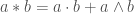
The other thing I have to explain is how vector multiplication works: In geometric algebra, the vector product is defined as the dot product plus the wedge product:

$a*b = a \cdot b + a \wedge b$

The result of the dot product $a \cdot b$ is a scalar, and the result of the wedge product $a \wedge b$ is a bivector. So how do we add a scalar to a bivector? We don’t, we just leave them as is. It works the same way as when adding polynomials $2x + 4x^2$ or when adding apples and oranges $3 apples + 4 oranges$ or when working with complex numbers: $5 - 2i$ . We just leave both terms.

Note that usually I will leave out the star and just write $a*b = ab$ .

In 3D space we have three basis vectors:

$x = (1, 0, 0)$

$y = (0, 1, 0)$

$z = (0, 0, 1)$

When multiplying these with each other we notice three properties of this new way of multiplying:

$xx = x\cdot x + x \wedge x = 1 + 0 = 1$

$xy = x\cdot y + x \wedge y = 0 + x \wedge y = x \wedge y$

$yx = y \cdot x + y \wedge x = 0 + y \wedge x = y \wedge x = -x \wedge y = -xy$

So when multiplying the basis vectors with each other, either the dot product or the wedge product is zero. We are left only with one of the two.

All other vectors can be expressed using the basis vectors. So the vector $(10, 5, 0)$ can also be written as $10x + 5y$ and I will use the second notation more often, because it makes multiplication easier.

With that out of the way, we can finally give one real example of how vector multiplication works in geometric algebra. It’s actually pretty simple because we just multiply every component with every other component:

$(10x + 5y) * (3x + y) = (10x * 3x + 10x * y + 5y * 3x + 5y*y)$

$= (30x^2 + 10xy + 15yx + 5y^2)$

$= (30 + 10xy - 15xy + 5)$

$= (35 - 5xy)$

Let’s walk through a few of the steps I did there:

$10x*3x = 30x^2 = 30$ because $xx = x \cdot x + x \wedge x = 1 + 0 = 1$ .
$10x * y = 10xy$ because $xy = x \cdot y + x \wedge y = 0 + x \wedge y$ , so the scalar part is zero, and can write the wedge product of basis-vectors shorter as $x \wedge y = xy$ . This short-hand notation is only valid for vectors which are orthogonal to each other.
$5y*3x = 15yx = -15xy$ because $yx = y \cdot x + y\wedge x = 0 + y \wedge x = -x \wedge y = -xy$

So as promised the result of multiplying two vectors is a scalar ( $35$ ) and a bivector ( $-5xy$ ). A sum of different components like this is called a multivector.

When doing these multiplications you quickly notice that just as all vectors can be represented as combinations of $x$ , $y$ and $z$ , all bivectors can be represented as combinations of $xy$ , $yz$ and $zx$ . So I’ll just use these as my basis-bivectors. We could make different choices here, for example we could use $xz$ instead of $zx$ but I like how the bivectors circle around like that. The choice of bivectors doesn’t really matter, just as the choice of basis-vectors doesn’t really matter. We could for example have also chosen $x$ , $y$ and $-z$ as our basis vectors. All the math works out the same, we just get different signs in a few places.

Once we have three basis-vectors and three basis-bivectors, we notice that we can represent all 3D multivectors as combinations of 8 numbers: 1 scalar, 3 vector-coefficients, 3 bivector-coefficients and 1 trivector-coefficient. If we did the same exercise in a different number of dimensions, we would find similar sets of numbers. In 2D space for example we have 1 scalar, 2 vector-coefficients and 1 bivector-coefficient. That makes sense, because in 2D there are only 2 directions, only 1 plane and no trivector because there is no volume. If we went to 4D we would have 1 scalar, 4 vector-coefficients, 6 bivector-coefficients, 4 trivector-coefficients and 1 quadvector-coefficient. I’m sure you can spot the pattern that would allow you to go to any number of dimensions. (but really these come out naturally depending on how many orthogonal basis-vectors you start with)

We’re almost finished with our introduction to geometric algebra, so I need to mention one final important property: vector multiplication is associative. Meaning 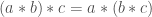$(a*b)*c = a*(b*c)$ so we can choose which multiplication we want to do first.

OK with that we’re finished with the introduction, but I want to practice a few more multiplications so that you get the hang of it. Maybe do a few yourself. It takes a couple minutes, but then you have the rules ingrained into muscle memory. This practice section is optional though.

Vector Multiplication Practice

Let’s do some practice runs to build up an intuition for how these vectors and bivectors behave. You can skip this section entirely if you don’t care about geometric algebra and just want to get to rotations.

What happens if we multiply two similar bivectors?

$2xy * 4xy = 8xyxy = 8x(yx)y = -8x(xy)y = -8(xx)yy = -8yy = -8$

So what I did there is I used $yx = -xy$ to re-order the basis-elements. Then everything collapses down because $xx = yy = 1$ . So what we see here is that the dot product of a bivector is a negative number. Isn’t that interesting? In particular if we have a bivector of length 1 and multiply it with itself: $1xy*1xy = xyxy = -xxyy = -1$ we see that $xy^2 = -1$ . Remember how in quaternions there are these three components $i$ , $j$ and $k$ which have $i^2 = j^2 = k^2 = -1$ ? We’re going to be using the bivectors for that. However it just so happens that the bivector is a mathematical construct whose square is -1. That does not mean that it is the result of $\sqrt{-1}$ . I could build any number of mathematical constructs that square to -1, (for example trivectors also square to minus one) that doesn’t mean that they are all the square root of -1. How many square roots is -1 supposed to have?

Speaking of squaring a trivector, let’s try that to get practice at re-ordering these components:

$xyz*xyz = xyzxyz = -xyxzyz = xxyzyz = yzyz = -yyzz = -zz = -1$

Getting the hang of it yet? It’s all about re-ordering components until things collapse.

Let’s try multiplying two different bivectors:

$xy * zx = xyzx = -xyxz = xxyz = yz$

The result of two bivectors is another bivector. If we have more complicated bivectors that are made up of multiple basis-bivectors, the result is a scalar plus a bivector:

$(2xy - 2yz) * (5yz + 0.5zx) = 2xy*5yz + 2xy * 0.5zx - 2yz * 5yz - 2yz * 0.5zx$

$= 10xyyz + xyzx - 10yzyz - yzzx$

$= 10xz + yz + 10 - yx$

$= 10 + xy + yz - 10zx$

So this is a scalar ( $10$ ) plus quite a complicated bivector ( $xy+yz -10zx$ ).

What happens if we multiply across dimension. Like multiplying a vector with a bivector?

$xy * 2x = 2xyx = -2xxy = -2y$

If we multiply the plane with a vector that’s on the plane, we get another vector on the plane. In fact if we do this a few more times:

$xy * -2y = -2xyy = -2x$

$xy * -2x = -2xyx = 2xxy = 2y$

$xy * 2y = 2xyy = 2x$

We notice that after four multiplications we are back at the original vector $2x$ . So every multiplication with a bivector rotates by 90 degrees. If we multiply on the left side instead of multiplying on the right side, we would rotate in the other direction.

What if we multiply the plane with a vector that’s orthogonal to it?

$xy * z = xyz$

Well that’s disappointing, we just get the trivector. What if we multiply the trivector with the plane?

$xyz * xy = xyzxy = -xyxzy = xxyzy = yzy = -yyz = -z$

If we multiply the trivector with the plane, the plane collapses and we’re left with just the vector that’s normal to the plane. This works even for more complicated bivectors:

$xyz * (0.707xy + 0.707zx) = 0.707xyzxy + 0.707xyzzx = -0.707z - 0.707y$

Which is the normal of the original plane. What if we multiply a vector with the trivector?

$xyz * x = xyzx = yz$

If we multiply a vector with the trivector, the vector part collapses out and we’re left with the plane that the vector is normal to. This works even for more complicated vectors:

$xyz * (-0.707y - 0.707z) = -0.707xyzy - 0.707xyzz = -0.707zx - 0.707xy$

And with that we’re back at the original plane. Almost. The sign got flipped. If we had multiplied by $-xyz$ we would have been back at the original plane.

So multiplying with the trivector turns planes into normals and normals into planes, because the other dimensions collapse out. This also allows us to define the cross product in geometric algebra: $a\times b = -xyz*a\wedge b$ . So first we build a plane by doing the wedge product, then we get the normal by multiplying with the trivector.

Reflections

If you went through the practice chapter you will have already seen places where geometric algebra does rotations: bivectors rotate vectors on their plane by 90 degrees. It’s not quite clear how we can build arbitrary rotations with that though.

One thing that’s a little bit easier to do is reflections, and we will see that we can get from reflections to rotations.

Let’s say we want to reflect the vector a in the picture below on the normalized vector r, to get the resulting vector b:

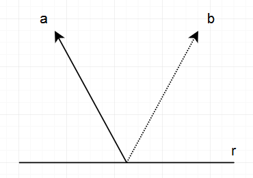
To do that it’s useful to break the vector a into two parts: The part that’s parallel to r, $a_\|$ and the part that’s perpendicular to r, $a_\perp$ :

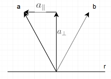
(forgive my crappy graphing skills)

These have a few properties:

$a = a_\| + a_\perp$

$a_\| *r = r*a_\|$ (the result is a scalar and we can flip the order)

$a_\perp* r = -r *a_\perp$ (the result is a bivector and flipping the order flips the sign)

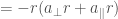
From the picture it should be clear that if we subtract $a_\|$ instead of adding it, we should get to $b$ . Or in other words:

$b = a - 2a_\|$

$= a_\| + a_\perp - 2a_\|$

$= a_\perp - a_\|$

So how do we get these $a_\|$ and $a_\perp$ vectors? You may already know how to do it, but we actually never need to explicitly calculate them. Because we can actually represent this reflection as

$b = -rar$

How do we get to that magical formula? Let’s multiply it out:

$-rar = -r(a_\perp + a_\|)r$

$= -r(a_\perp r + a_\|r)$

$= -ra_\perp r - ra_\|r$

$= r^2a_\perp - r^2a_\|$

$= a_\perp - a_\|$

The important step is that $a_\perp r = -ra_\perp$ , allowing us to re-order the elements until we’re left with $r^2 = r\cdot r$ which is just 1, as long as $r$ is normalized.

Rotations

The reflections above look kinda like rotations. In fact if all we want to do is rotate a single vector, we can always do that with a reflection. The problem is if we want to rotate multiple vectors, like in a 3d model, then the rotated model would be a mirror version of the original model.

The solution to that is to do a second reflection. There are many possible pairs of reflections that we could choose, but here is an easy one. First we reflect on the half-way vector between $a$ and $b$ , $r=\frac{a+b}{|a+b|}$ (where writing pipes around a vector like $|v|$ is the length of the vector, so $\frac{v}{|v|}$ is a normalized vector):

rotate_half

So in this picture I am reflecting $a$ on the vector $r$ , which is half-way between $a$ and $b$ , landing us at $-b$ . To get from $-b$ to $b$ we just have to do a second reflection with the vector $b$ itself. (which is a bit weird, but if you follow the equations it works out) Given that $-rar$ is one reflection, $brarb$ is two reflections. First we reflect on $r$ , then we reflect on $b$ .

Earlier we chose $r = \frac{a+b}{|a+b|}$ . We can multiply this out and define

$R = b\frac{a+b}{|a+b|}$

$= \frac{ba + 1}{|a+b|}$

Then the rotation is written as $b=Ra\overline R$ (where you could work out $\overline R$ by multiplying out the other side, or you can just flip the sign on the bivector parts of $R$ ), and the inverse is written as $a=\overline RbR$ .

Quaternions

And just like that we have quaternions. How? Where? I hear you asking. That $R$ part in the last equation is a quaternion. If you multiply it all out, you will find that all the vector parts and trivector parts collapse to 0, and you’re just left with the scalar part and the bivector coefficients. And it just so happens that if you have a multivector which consists of only a scalar and the bivectors, multiplication behaves exactly like multiplication of quaternions.

Now isn’t that interesting? All we did was we did the math for reflections, and if we do two of those we get quaternions? No imaginary numbers, no fourth dimension, just 3d vector math. All we had to do was introduce that wedge product $a \wedge b$ .

And you’ll notice that the way we apply $R$ , by doing $Ra\overline R$ looks an awful lot like how we multiply quaternions with vectors. To multiply a quaternion $q$ with a vector $a$ we do $q*(0, a)*\overline q$ .

OK so let’s convince ourselves that these really are quaternions and work out the quaternion equations. They are 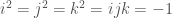$i^2=j^2=k^2=ijk=-1$ . Our quaternion consists of a scalar and three bivectors, $yz$ , $zx$ , and $xy$ . (I use them in this order because the $yz$ plane rotates around the x axis, so it should come first). So let’s try this:

$yz^2 = yzyz = -yyzz = -1$

$zx^2 = zxzx = -zzxx = -1$

$xy^2 = xyxy = -xxyy = -1$ .

Seems to work so far. But I actually don’t fulfill the equation $ijk = -1$ because for me $yz*zx*xy = yzzxxy = yy = 1$ . I could fix that by choosing a different set of basis-bivectors. For example if I chose $yz$ , $xz$ and $xy$ , then this would work out because $yz*xz*xy = yzxzxy = -yzzxxy = -yy = -1$ . But I kinda like my choice of basis vectors and all the rotations work out the same way. If this bothers you, just choose different basis bivectors.

One super cool thing is that when doing the derivations using reflections, I never had to specify the number of dimensions. We could use 3D vectors or 2D vectors or any number of dimensions. So if we work out the math in 2D, what do you think we get? That’s right, we get complex numbers: One scalar and one bivector. Because that’s how you do rotations in 2D. But we could go to any number of dimensions using this method. (except in 1D this kinda collapses, because you can’t really rotate things in 1D)

Also we didn’t specify what we are rotating. We assumed that it was a vector, but we never required that. So this can rotate bivectors and it can rotate other quaternions.

Interpreting Geometric Algebra Quaternions

So we found a new way to derive quaternions. This new way is neat because we don’t need 4 dimensions and we don’t need imaginary numbers. But can we learn anything new from this? Already we have two possible new interpretations:

A quaternion is the result of two reflections
A quaternion is a scalar plus three bivectors

Maybe one of these has some interesting conclusions.

Before that I want to kill the 4D interpretation properly: There are two reasons why people say quaternions are 4D: The fact that quaternions have four numbers, and the fact that quaternions have double cover. I’ll talk about the double cover separately later, but here I briefly want to talk about the four numbers thing. There are lots of 3D constructs that have more than three numbers. For example a plane equation has four numbers: 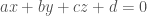$ax+by+cz+d = 0$ . Or if we want to do rotations using matrices in 3D, we need a 3×3 matrix. That’s 9 numbers. But nobody would ever suggest that we should think of a rotation matrix as a 9 dimensional hyper-cube with rounded edges of radius 3. So don’t think of quaternions as a 4 dimensional hypersphere of radius 1. Yes, there are some useful conclusions to draw from that interpretation (for example it explains why we have to use slerp instead of lerp) but it’s such a weird interpretation that it should come up very rarely.

With that out of the way let’s get to these two new interpretations:

1. Interpreting quaternions as two reflections. I couldn’t get much useful out of this. The first reflection is always on the vector half-way between the start of the rotation and the end of the rotation. The second reflection is always on the end of the rotation. I’ve played around with visualizing that, but the visualizations always looked predictable and didn’t offer any insights.

2. Interpreting quaternions as a scalar plus three bivectors. This interpretation on the other hand turned out to be a goldmine. Not only can you get an intuitive feeling for how this behaves, you can also get visualizations from this. This interpretation also allowed me to get rid of the double cover of quaternions.

So even though we have derived quaternions using reflections above, I will actually spend the rest of the blog post talking about quaternions as scalars and bivectors.

Scalars and Bivectors

A quaternion is made up of a scalar and three bivectors. We all know what a scalar does: Multiplying with a scalar makes a vector longer or shorter. I said above that multiplying with a bivector rotates a vector by 90 degrees on the plane of the bivector.

So how can we build up all possible rotations if all we have is a scalar and three rotations of exactly 90 degrees? The answer is that a bivector actually does slightly more: It rotates by 90 degrees, and then scales the vector.

I said that a bivector is a plane. But because of its rotating behavior, I actually like to visualize it as a curved line. So I visualize a vector as a straight line, and a bivector as a 90 degree curve. So here is a visualization of three different bivectors:

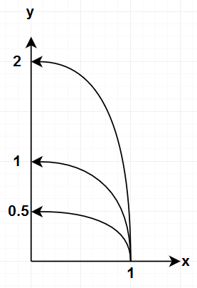
These are the bivectors $0.5xy$ (bottom), $xy$ (middle) and $2xy$ (top). It’s a 90 degree rotation followed by a scale. I find this visualization particularly useful when chaining a bunch of operations together.

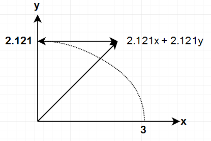
For example let’s say we want to rotate by 45 degrees on the xy plane. To do that we can multiply a vector with the quaternion $0.707 + 0.707xy$ . (that 0.707 is actually $\frac{1}{\sqrt{2}}$ , but I’ll truncate it to 0.707 here) Now let’s multiply the vector $3x$ with that quaternion. That gives us

$3x * (0.707 + 0.707xy) = 2.121x + 2.121y$

Here’s how I would visualize that:

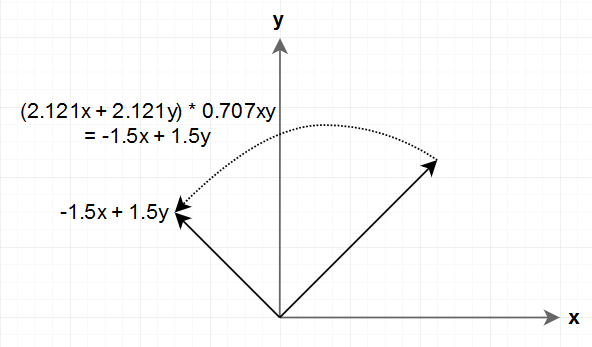
First we rotate by the bivector to get $2.121y$ :

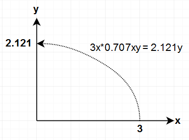
So the bivector is a rotation by 90 degrees followed by a scale of 0.707.

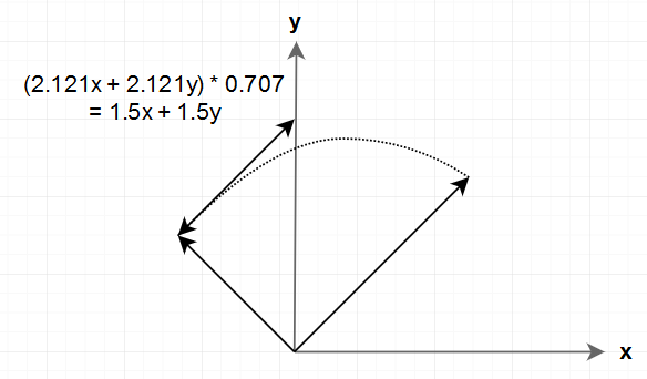
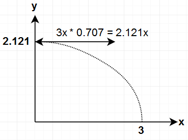
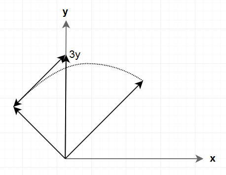
Next we multiply the original vector with the scalar to get the vector $2.121x$ , which we add to the previous result:

Which then gives us the final vector of 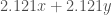$2.121x + 2.121y$ :

Which is the original vector rotated by 45 degrees.

This way of visualizing makes it very clear that multiplication with a quaternion is just multiplication with a scalar and multiplication with a bivector. And this also shows how we got a 45 degree rotation, even though all we can do is 90 degree rotations followed by scaling. It also explains why we need the single scalar value, and why the three bivectors are not enough: We sometimes want to add some of the original vector back in to get the desired rotation.

One thing to note is that in here I chose to do the bivector multiplication first, and the scalar multiplication second. But the choice is kinda arbitrary as both of these happen at the same time, and they don’t depend on each other.

Let’s rotate that same vector again to show what this looks like when we didn’t start off with one of our basis vectors:

$(2.121x + 2.121y) * (0.707 + 0.707xy) = 2.121x*0.707 + 2.121x * 0.707xy + 2.121y * 0.707 + 2.121y * 0.707xy$

$= 1.5x + 1.5xxy + 1.5y + 1.5yxy$

$= 1.5x + 1.5y + 1.5y - 1.5x$

$= 3y$

So let’s visualize that:

First we rotate with the bivector, which puts us at $-1.5x + 1.5y$ :

So once again this does a 90 degree rotation followed by a scale of 0.707.

Next we multiply the original vector by 0.707 and add the resulting vector $1.5x + 1.5y$ :

Which then gives us the final vector of $3y$ :

Which is exactly what we would expect after rotating by 45 degrees twice.

I think these visualizations also explain how we can get arbitrary rotations: For bigger rotations we just have to make the scalar component smaller as the bivector component gets bigger.

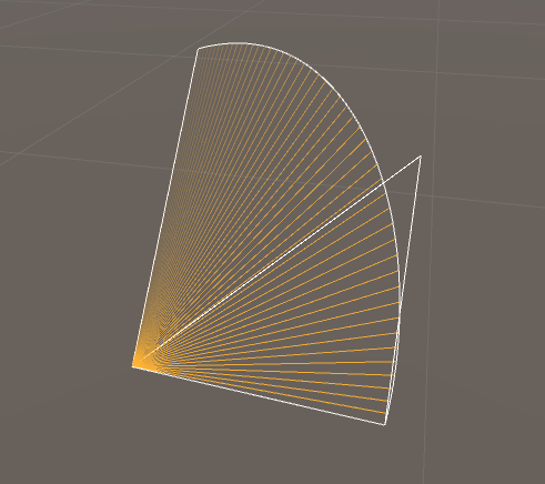
So far we have only looked at the xy plane. To visualize this in 3D, I wrote a small program in Unity that can do the above visualization for all three bivectors. Here is what that looks like for rotating from the vector 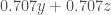$0.707y + 0.707z$ to the vector $0.707x + 0.707y$ . That gives me the particularly nice quaternion $0.5 - 0.5yz + 0.5zx - 0.5xy$ .

This is going to be hard to do in pictures because it’s a 3D construct, but I’ll give it a shot. Here is what the two vectors look like:

So I want to rotate from the vector on the left to the vector on the right.

Here is what the contribution of the $-0.5xy$ bivector looks like:

unity_vectors2_xy

So this bivector is rotating on the xy plane. It takes the end point of the vector and rotates it 90 degrees down on the xy plane. It may be a bit hard to see, but imagine all the yellow lines lying on a xy plane.

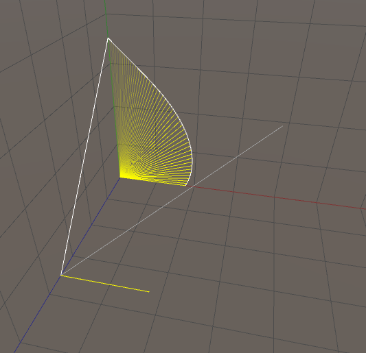
The result of that 90 degree rotation is the vector $0.353x$ . (the lower edge of the plane) I used the end of that rotation to start our result vector. (see how I have a third short vector sticking out at the bottom now? That’s $0.353x$ )

Next I’m doing the contribution of the $-0.5yz$ bivector:

The original vector was already rotated 45 degrees on the yz plane, so this rotation started off at a 45 degree angle and it rotated 90 degrees on the yz plane. Then it scaled the result by 0.5, giving us the result vector $0.353y - 0.353z$ . (the bottom of the teal plane)

I also added the result of that rotation to the result vector. (the shorter vector that was sticking out now has a corner in it, indicating that I added the new $0.353y - 0.353z$ )

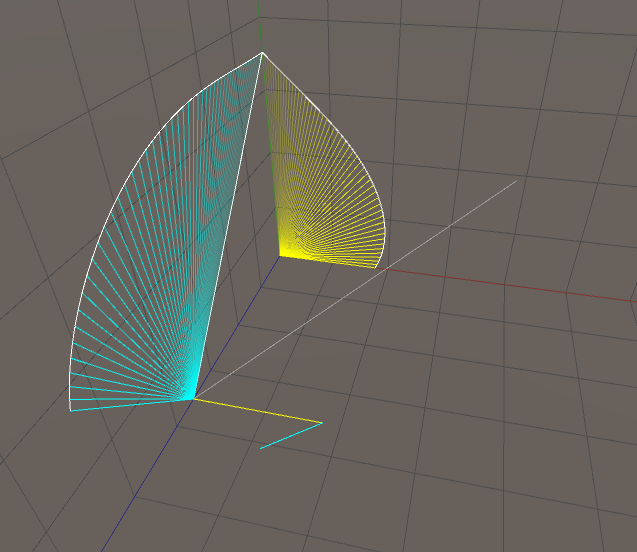
Next we add the contribution of the $0.5 zx$ bivector:

This took the end point of the original vector, and rotated it by 90 degrees on the zx plane. Then it scaled the result by 0.5, giving us the new vector $0.353x$ (the end of the purple plane). The reason why the purple plane is floating above the other planes is an artifact of my visualization: I start at the end point and then I only move on the zx plane, so I end up floating above everything else. I also added this to our result vector at the bottom there.

Finally I’m going to add the $0.5$ scalar component into this:

This just took the original vector and scaled it by 0.5, giving us $0.353y + 0.353z$ . I then added that to the results of the three bivector rotations. And as we can see, if we add up the contributions of the three bivectors and of the scalar part, we end up exactly at the end point of the vector that we were rotating into. (it may look like the last part is longer than 0.5 times the original vector, but that’s a trick of the perspective. The reason I picked this perspective is that you can see all three rotations from this angle)

So the rotation happened by doing three bivector multiplications and one scalar multiplication and adding all the results up.

Once again I want to point out that the order in which I added these up is arbitrary. All of these multiplications happen at the same time and don’t depend on each other, since they all just use the original vector as input. I chose to do this in the order xy, yz, zx, scalar, because that gave me a nice visualization.

I wanted to make the above visualization available for you to play with. I thought I could be really cool and upload a webgl version so that you can just play with it in your browser. So I built a webgl version, but then I found out that I can’t upload that to my wordpress account. So… I just put it in a zip file which you have to download and then open locally… Here it is.

There is an alternate visualization for the above rotation: Just as we would think of the vector $10x + 5y$ as a single vector, we can also think of the bivector $-0.5yz + 0.5zx - 0.5xy$ as a single bivector. It’s the plane with the normal $-0.5x + 0.5y - 0.5z$ , which is the plane spanned between the start vector and the end vector of the rotation. Then the visualization shows a 90 degree rotation on that plane, followed by a scaling of the length of this bivector. (which is $\sqrt{0.5^2 + 0.5^2 + 0.5^2} = 0.866$ ) That visualization looks like this:

So we rotate on this shared plane, then scale by 0.866, and finally add the original vector scaled by 0.5. This visualization as a single 90 degree rotation by the sum-bivector is equally valid as the visualization of the component bivectors. Just as we can visualize vectors either by their components, or as one line, we can visualize bivectors either by their components or as a single plane.

That finishes the part about visualization. As far as I know this is the first quaternion visualization that doesn’t try to visualize them as 4D constructs, and I think that really helps. Every component now has a distinct meaning and a picture. And we can see how the behavior of the whole quaternion is a sum of the behavior of its components.

Axis Angle

One quick aside I want to make is that sometimes people say that quaternions are related to the axis/angle representation of rotations. That is a good way to get people started with quaternions, but then it breaks down relatively quickly because the equations don’t make sense and the numbers behave weirdly. The scalar & bivector interpretation is actually related to the axis/angle interpretation, and it explains what’s really going on here. Because when I say that something rotates 90 degrees on a plane, we can also say that it rotates 90 degrees around the normal of the plane. So in this interpretation quaternions first: rotate 90 degrees around the normal, followed by being scaled down, and second: multiply the original vector times a scalar and add that. It’s not quite axis/angle, but we can see how it’s related and why the axis/angle interpretation sometimes seems to work.

With the scalar & bivector interpretation of quaternions, we have a good idea of what quaternions do. With that, we’re ready to tackle the final quaternion mystery:

Quaternion Double Cover

When I was working on this, a few friends asked me how the “scalar and bivector” explanation explains the double cover of quaternions. If you’re not familiar, the double cover means that for any desired rotation, there are actually two quaternions that represent that rotation. For example the quaternions that have 1 or -1 in the scalar part, and 0 for all the bivectors both represent a rotation by 0 degrees. (or by 360 degrees depending on how you look at it)

At first I responded that I hadn’t gotten to that part yet, but as I was working on this, the double cover just never came up. So eventually I decided to go looking for it, and… I couldn’t find it. It seemed like my quaternions didn’t have double cover. So I double checked everything and noticed that I have one difference: Remember how in order to multiply a quaternion $R$ with a vector $v$ we did this multiplication: $Rv\overline R$ . I accidentally didn’t do that. I just did $Rv$ .

And the simple multiplication actually works as long as you’re only rotating vectors on a plane that they actually lie on. For example rotating the vector $x$ on the $xy$ plane works out: $xy*x = -y$ . The problems start if we’re rotating a vector that doesn’t completely lie on the plane that you’re rotating on. So let’s say I’m rotating the vector $2x + 2z$ on the $xy$ plane:

$xy(2x + 2z) = 2xyx + 2xyz$

$= -2y + 2xyz$

That’s strange: Some of our vector part has disappeared, and instead we have a trivector. This is not good. You don’t want part of the vector to disappear after a rotation. Rotating with $Rv\overline R$ fixes the problem, because the trivector part cancels out:

$xy*(2x + 2z)*-xy = (2xyx + 2xyz)*-xy$

$= -2xyxxy - 2xyzxy$

$= -2x + 2z$

So now the part that’s on the plane (the $x$ component) got rotated, but the part that’s not on the plane (the $z$ component) was left unchanged. This is exactly what we want.

But look at what happened: The first rotation was a 90 degree rotation and the part that’s on the plane ended up at $-2y$ . And now we did a full 180 degree rotation and that part ended up at $-2x$ . How did that happen?

Well it actually makes sense. We are multiplying with the quaternion twice after all. Of course it would do a double rotation. It’s clearest if you multiply it all out, but the short explanation is that the conjugate allows us to rotate roughly in the same direction while multiplying from the other side: $Ra \approx a\overline R$ , and we went ahead and just multiplied on both sides $Ra\overline R$ . So if we multiply on both sides of course we get twice the rotation.

This is literally where the half-angles of quaternions and the double cover come from: From the way we multiply quaternions with vectors. Internally quaternions actually don’t have double cover. If you multiply one 90 degree quaternion with a different quaternion, then after four rotations that second quaternion will end up exactly where it started. But then we chose a vector multiplication function that applies the quaternion twice. So we have to change the interpretation and that 90 degree quaternion becomes a 180 degree quaternion. And actually my visualizations above don’t make sense any more because the vector multiplication always does that operation twice.

Killing Double Cover

So if the vector multiplication is the problem, could we define a vector multiplication that doesn’t lead to double cover? That would make quaternions much simpler.

And the answer is that yes, we can. Remember that rotating vectors that lie on the plane already worked correctly. The problem was that rotating an orthogonal vector would turn into a trivector. (but rotations should leave orthogonal vectors unchanged) The solution is that we have to first project the vector down onto the plane, then rotate within the plane, and then apply the original offset again. Here is an outline of the algorithm:

Compute the normal of the plane by multiplying with the trivector (very fast)
Project the vector onto that normal (fast, as long as you use the version without a square root)
Subtract that projected part (very fast)
Multiply the vector with the quaternion
Add the projected part (very fast)

So now we only have to do a single multiplication instead of two multiplications. And since all other operations are fast, this might even be faster than the double-cover-giving quaternion/vector multiplication.

And yes, this totally works and it’s faster and it’s less confusing. But you don’t want to use it. The reason is that as soon as I didn’t have double cover in my quaternions, I discovered why double cover is actually awesome.

Why We Need Double Cover

Double cover is what makes quaternion interpolation so great. (by interpolation I mean getting from rotation a to rotation b in multiple small steps as opposed to one large step) Without double cover, there are some quaternions that you can not interpolate between. Having to worry about those special cases makes interpolation a giant pain and defeats the whole point of why we used quaternions to begin with.

To explain what the problem is, let’s do a couple 90 degree rotations on the $xy$ plane, once using double cover and once not using double cover:

Rotation	Single Cover	Double Cover
$0^\circ$	$1 + 0xy$	$1 + 0xy$
$90^\circ$	$0 + xy$	$0.707 + 0.707xy$
$180^\circ$	$-1 + 0xy$	$0 + xy$
$270^\circ$	$0 - xy$	$-0.707 + 0.707xy$
$360^\circ$	$1 + 0xy$	$-1 + 0xy$

If we interpreted these two numbers as vectors, the double cover version would do a 45 degree rotations of the vector each time. But since the double cover quaternion will rotate twice, this will actually give us a 90 degree rotation from one row to the next.

Here is a visualization of the same numbers. The idea here is that I put the scalar value on the x axis and the $xy$ bivector on the y axis:

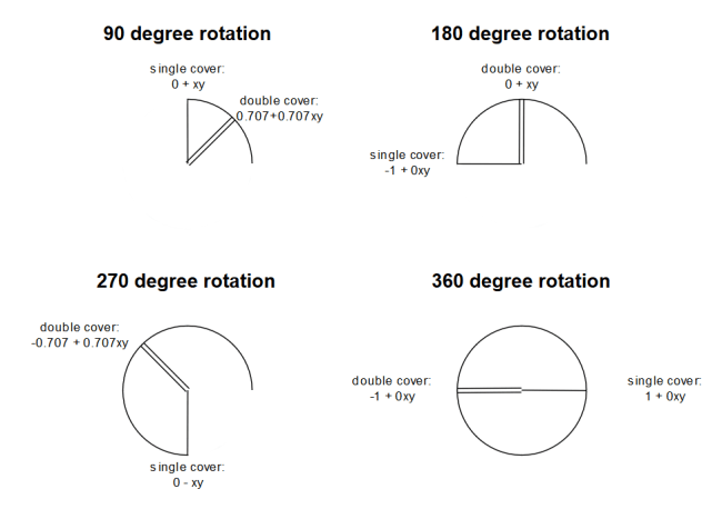
I drew the double cover as two lines, and the single cover as one line. Once again we see that a quaternion that uses double cover rotation is simply half-way towards the quaternion that uses single cover rotation.

I said that double cover is what makes quaternion interpolation so great. To see why, let’s try interpolating between these. To keep it simple I won’t do a slerp, but I’ll just try to find the rotation half-way between any of these rotations. We do that by adding the quaternions and then renormalizing them. Interpolating from the $0^\circ$ rotation to the $90^\circ$ rotation is pretty easy in both cases:

For single cover: $(1 + 0xy) + (0 + xy) = 1 + xy$ and after normalization that comes out to be $0.707 + 0.707xy$ which is a 45 degree rotation.

For double cover: $(1 + 0xy) + (0.707 + 0.707xy) = 1.707 + 0.707xy$ and after normalization that comes out to be $0.924 + 0.383xy$ , which is a 22.5 degree rotation, or with the double cover it’s a 45 degree rotation.

So interpolating a 90 degree rotation works just fine in both cases.

However we run into problems when interpolating from the $0^\circ$ rotation to the $180^\circ$ rotation:

For single cover: $(1 + 0xy) + (-1 + 0xy) = 0$ . Huh. We can’t find the half-way rotation between these two because we just get 0, which we can’t normalize. You may think that this is just a problem because I chose to find the exact midpoint between these two vectors. But this is also a problem if we want to slerp from one to the other. It all collapses and we’re left with a zero vector.

So let’s reason through this manually. How would we interpolate from +1 to -1? We could rotate on the xy plane or on the yz plane or on the zx plane, or on any combined bivector. How do we know which bivector to choose? They’re all zero in both of our inputs. We’re missing information. In order to interpolate between two rotations, we need to know a plane on which we want to interpolate.

Let’s see how the double cover solves this: $(1 + 0xy) + (0 + xy) = 1 + xy$ and after normalization we’re left with $0.707 + 0.707xy$ which was our 90 degree rotation, which is exactly the half-way point between the 0 degree rotation and the 180 degree rotation.

Isn’t that neat? In the double cover version one of our quaternions had a $xy$ component, so we could interpolate on that plane. In fact you could build many possible 180 degree rotations in the double cover version. We could build a 180 degree rotation that rotates on the $yz$ plane or on a linear combination of the $xy$ and $zx$ planes, or on any arbitrary plane. They all look different and they all interpolate differently. That’s a great property because we want to be able to interpolate on any plane of our choosing. In the single cover version however we only have one way to rotate 180 degrees and it looks the same no matter which plane you’re on. Which works fine if all you want to do is rotate 180 degrees, but it doesn’t work if you want to interpolate from one rotation to the other.

One way of thinking of this is that the trick of double cover is that you can express any rotation as a rotation of less than 90 degrees. We already saw that if we want to go 180 degrees, we just go 90 degrees twice. Want to go 270 degrees? Just go -45 degrees twice. Like that we can always stay far away from the problem point of the 180 degree rotation that we would run into often if we used the single cover version of quaternions. And like that we always keep the information of which plane we are rotating on, making interpolation easy.

Another way of thinking of this is that the double cover version always gives us a midpoint of the rotation which we can use to interpolate. For some pairs of rotations, there are a lot of possible midpoints depending on which plane we want to interpolate on. Double cover solves that problem by giving us one midpoint, which narrows our choices down to one plane. And we can derive any other desired interpolation if we have the midpoint.

You may be wondering if there is a problem point where the double cover breaks down. Looking at the table above, we can find one: Rotating by 360 degrees: $(1 + 0xy) + (-1 + 0xy) = 0$ . Which we can not renormalize. But that case is easy to handle, and in fact every slerp implementation already handles this: We detect if the dot product of the quaternions is negative, and if it is we flip the target quaternion. So then we interpolate from $(1 + 0xy)$ to $(1 + 0xy)$ which is just a 0 degree rotation. Which is exactly what we wanted. So as long as we handle the “negative dot product” case in our interpolation function, we can handle all possible rotations. Because there are two possible ways to express every rotation, and if we run into one that’s inconvenient, we just switch to the other one.

So I hope I have convinced you that you want to have double cover. It’s a neat trick that makes interpolation easy. Quaternions do not “naturally” have double cover, but the double cover comes from the way we define the vector multiplication. If we used a different algorithm to multiply a quaternion with a vector (I outlined one above) then we could get rid of the double cover, but we would be making interpolation more difficult. I actually think that the double cover trick is not unique to quaternions. I think we could also apply it to rotation matrices to make them easier to interpolate. I haven’t done the math for that though.

Summary

So in summary I hope that I was able to make quaternions a whole lot less weird. The geometric algebra interpretation of quaternions shows us that they are normal 3D constructs, not weird four-dimensional beasts. They consist of a scalar and three bivectors. Bivectors do 90 degree rotations followed by scaling, and we saw how we can create any rotation just from those 90 degree rotations and linear scaling. The rules that govern these constructs are simple, making the equations easy to derive and understand. (as opposed to the quaternion equations which can only be memorized) Also quaternions do not naturally have a double cover. The double cover comes from the way we define the multiplication of vectors and quaternions. We could get rid of it, but the double cover is a great trick for making interpolations easier.

Unfortunately this still only makes it slightly easier to understand the numbers in quaternion. The double cover makes it so that each rotation actually gets applied twice, so my visualizations above only show half of what’s going on. This also makes it difficult to interpret the numbers because you have to know what happens if a rotation gets applied twice, which is a whole lot harder to do in your head than doing a single rotation. But still I now have a picture of quaternions, and I know what each component means, and why they behave the way they do. I hope I was able to do something similar for you.

I also think that Geometric Algebra is a very interesting field that merits further study. The fact that quaternions came out so naturally (in fact they almost don’t even need a special name) and that if we do the same derivation in 2D we end up with complex numbers is fascinating to me. The paper I linked at the beginning, Imaginary Numbers are not Real, spends a lot of time talking about how various equations in physics come out much simpler if we use geometric algebra instead of imaginary numbers and matrices. Simplicity like that is a good hint that there is something good going on here. If you’re interested in this for doing 3D math, there is something called Conformal Geometric Algebra which adds translation to quaternions. I didn’t look too much into it, but a brief glance shows that it might be related to dual quaternions. So there’s much more to discover.

18 Comments to “Less Weird Quaternions”

ioquatix says:

August 7, 2017 at 07:38

The cross product also works in 4D and up.

- Malte Skarupke says:
  
  August 7, 2017 at 09:17
  
  Interesting, I didn’t know that. I can see how the geometric algebra version works in 4D. I think it would return a bivector (plane) instead of a vector. But I didn’t know that the normal cross product works in 4D. Can you elaborate?
  
  - troyip says:
    
    August 7, 2017 at 11:51
    
    ioquatix is only half-right. The cross product that we know and love only works in 3D and 7D. It is only in these dimensions that the cross product results in a vector that is orthogonal to the others.
    
    You “can” make something that looks like a cross product in other dimensions, but the result won’t be linearly independent to the vectors you started with.
Edward Kmett says:

August 7, 2017 at 19:50

In general when talking about a quadratic space (a vector space with an associated quadratic form we use to “measure” vectors) we look at its signature and say if we were to diagonalize this quadratic form and with an appropriate change of basis, e.g. replacing Q with A^-1DA with D a diagonal matrix what would the signs of the things on the diagonal of D be? This gives us a signature of sorts R^(a,b,c) where a is the number of positive items on the diagonal and b is the number of negative items on the diagonal and c is the number of zeroes on the diagonal.

Dual numbers (and hence dual quaternions) require a dimension that squares to 0. Dual quaternions live in R^(3,0,1). Adding an infinitesimal (dimension that squares to 0) is basically doing the same thing as automatic differentiation is doing. You can view dual quaternions equivalently as quaternions on dual numbers, or quaternion-valued dual numbers and it can be worthwhile to flip between those viewpoints.

On the other hand, conformal GA is basically about adding dimensions that square to negative values and using them to enrich your geometric algebra to cover circles and spheres.

toto says:

August 9, 2017 at 03:41

Hi, About the Unity Web GL app, is there any reason why you don’t publish it to something like Github? It will have 2 advantages : People would be able to see the code for the maths and you can publish the app to Github pages removing the need to download and open a zip.

Neb says:

August 10, 2017 at 11:25

Thank you for writing this. I have been trying to learn Geometric Algebra for a while and had been stuck, and your explanation got the things going again. I was working with surface normals, which make more sense as an embedding of bivectors into the original vector space. I feel I got the quaternions for free 🙂

Thank you so so much. You made my week.

not even three quarter says:

September 14, 2017 at 16:36

Brilliant write-up, I wish more research projects would be presented like this!

I do not share your enthusiasm for double cover though, the numbers are ugly and we _still_ have to special case n*360° …
If so, why not solve all the collapsing cases by some convention and stay single cover?

- Malte Skarupke says:
  
  September 16, 2017 at 14:57
  
  The double cover special case at 360 degrees is very easy to handle. We just don’t rotate at all in that case.
  
  The special case at 180 degrees that we get with single cover is not at all easy to handle. The reason is that when we rotate exactly 180 degrees, we don’t know which plane we should rotate on. All we can see is that the new direction is exactly the other way. But there is an infinite number of planes that we could rotate on in order to get there. So let’s say that our convention is that for 180 degree rotations we always rotate on the xy plane. Then let’s say I’m rotating in 1 degree steps on the yz plane. At 179 degrees I get an almost-halfway rotation on the yz plane. But if I do 1 more degree, all of a sudden it rotates on an entirely different plane. Meaning it rotates around a different axis.
  
  So if all we have is a 180 degree rotation, there is no convention that can handle all possible rotations. So we would need a convention that says “detect if you’re going to get a 180 degree rotation, and if you do just fudge it a little so that you get a 179.999 degree rotation instead.” And that might work. But it’s going to be messy.
  
  So double cover makes our lives a lot easier here by moving the special case to a point that’s easy to handle: Just don’t rotate at all when you hit the special case.
  
aduric says:

December 30, 2017 at 12:12

Hello, I’m in the process of learning about geometric algebra, and for me the best way to learn is to implement it in a programming language. Since I’m learning about Rust as well, I wrote a quick library that has basic geometric algebra objects and operations: https://github.com/aduric/cliff

Please let me know what you think. I would like to implement rotations next..

Looping rocks says:

March 15, 2018 at 05:18

There’s a nice conference where Chris Doran explains how he implemented GA in Haskell using “BitVectors”

https://skillsmatter.com/skillscasts/10772-geometric-algebra-in-haskell

He also provided the source code in the presentation notes

Looping rocks says:

March 15, 2018 at 05:22

Thanks for this nice introduction to 3D GA.

If I may, there’s a great ressource that gradually introduces GA from the basics to the advanced stuff. It has helped me greatly to grasp the full power of this framework.

https://www.visgraf.impa.br/Courses/ga/

Steven De Keninck says:

October 10, 2018 at 07:37

No doubt late to the party but to play with GA in all it’s shapes, in the browser, check out [ganja.js](https://GitHub.com/enkimute/ganja.js)

Joe says:

October 10, 2018 at 14:53

Wow, that was fascinating! Thanks very much for the article. The only thing I didn’t get was how the second step of a rotation was to reflect -b in b, is that something you can reasonably visualise or do you just have to do the maths to figure out out?

Joe says:

October 12, 2018 at 11:36

Something else I didn’t get – you say that

ab = a . b + a ^ b

Where a ^ b is a plane that both a and b occupy. However, when I do this multiplication I actually get a quaternion that rotates from a to b. So the bivectors resulting from the wedge product seem to be scaled by sin theta. Is that meant to be the case?

Andrzej Broński says:

April 6, 2019 at 07:39

Thank you for very detailed and intuitive explanation of quaternions!

Elliott Prechter says:

December 22, 2020 at 09:59

First off, this is one of the best posts I’ve read on Quaternions – thanks! Amazing work.

I do have some constructive feedback however that I’d also love to know if I’m right/wrong about.

Your post inspired me to try the “single cover” method of rotating a vector, and but I hit a snag.

First off, the “single cover” rotation works great when the Vector and the Rotor are co-planar (it’s actually just the dot product between them), which looks like this in C#:

public static Vec3 operator|( in Vec3 a, in Rotor3 b ) => new Vec3( a.Xb.A + a.Zb.ZX – a.Yb.XY, a.Yb.A + a.Xb.XY – a.Zb.YZ, a.Zb.A + a.Yb.YZ – a.X*b.ZX ); // dot (coplanar rotate ccw)

But when they’re NOT coplanar, we have to add back in the rejected part after doing the co-planar rotation, as you suggested:
```
// this does a coplanar rotation and adds back in the rejected part
public static Vec3 operator&( in Vec3 a, in Rotor3 b )
{
    var r = a.X*b.YZ + a.Y*b.ZX + a.Z*b.XY;
    return new Vec3(
        a.X*b.A + a.Z*b.ZX - a.Y*b.XY + r*b.YZ,
        a.Y*b.A + a.X*b.XY - a.Z*b.YZ + r*b.ZX,
        a.Z*b.A + a.Y*b.YZ - a.X*b.ZX + r*b.XY );
} // rotate ccw
```
Now, at first this new “coplanar rotate + add reject part” seemed to work for several test cases, until I hit a test case that broke it: what happens when you wan to rotate the Vector (1, 3, 5) by 180 degrees in the XY plane?

The rotor that does a 180 degree rotation looks like (-1, 0, 0, 0). This still works fine if the Vector is coplanar, but the Vector (1, 3, 5) is not coplanar. We can’t reject it against the XY plane though because the rotor’s bivector is NULL! So if you use the above method, you get the Vector (-1, -3, -5) after rotation, which is wrong.

So, without the double-cover concept, you actually lose information about the the plane of rotation when doing a 180 degree rotation. So double-cover isn’t just needed for interpolation, it’s needed just to do any rotation at all of non-coplanar vectors.

- Malte Skarupke says:
  
  January 17, 2021 at 19:26
  
  Thanks, this is a really good point. I mentioned how, when you lose the information about the plane of rotation, you can’t interpolate any more. But you’re correctly pointing out that the problem is much bigger: In this case you can’t rotate at all if the vector doesn’t lie on the plane. I don’t think there is a way to fix this, so that kills the single cover version entirely. They just don’t work in 3D or higher.
  
externo says:

December 29, 2023 at 11:11

I think the idea that (i,j,k) = (yz, xz, xy) is not good, because then i, j, k are spatial planes.
In quaternions, the scalar part represents time or density, it is not an arbitrary addition. In fact, (i,j,k) = (1x,1y,1z) i.e. the basis of space-time vectors. The scalar part is a dimension orthogonal to the other three, for this reason 1x <> x, it is a density vector and (1x)² = -1 = i². The vectors that are rotated in the quaternions are density vectors (they are combinations of i, j, k and not x, y, z). All quaternions whose scalar part is zero are vectors with homogeneous density (they are in the same time). If the scalar part is not zero, the density of the vector varies (it spans several epochs).
There are studies that are beginning to understand the true nature of quaternions, and this is not the same thing as what geometric algebra says, which apparently went astray by leaving aside the orthogonality nature of the scalar part. .
Here are two such physical studies :

Click to access 0307038.pdf

https://www.mdpi.com/2073-8994/15/9/1672
Such an approach requires abandoning the Einsteinian interpretation of relativity in favor of the Lorentizian interpretation.
https://en.wikipedia.org/wiki/Lorentz_ether_theory