Probably Dance

For the second time in my career, I ran into a problem where it’s actually useful to know how floating point numbers work. (first time was here) The problem is that sometimes you want floating point numbers that add well. So that you have the associativity guarantee that (a + b) + c == a + (b + c).

The use case here was for A* path finding, but this may also be applicable in other situations. I’ll explain a bit more of A* later, but as a motivation you just have to know that you can speed up A* a lot if you can reason about all the nodes in your graph that have the same “cost.” But since the “cost” is a sum of a lot of different floats, they will rarely have exactly the same value. At that point you could fudge numbers and say that “if two numbers are equal to within 0.0001, treat them as equal” but when you do that it’s easy to accidentally define an ordering that’s not a strict weak ordering. And I have literally seen a crash caused by an incorrect float ordering that was very rare and very hard to track down. So once bitten twice shy, I wanted to see if I couldn’t just force floating math to be exact. And turns out you often can.

To illustrate the problem in A* path finding, let’s start with a picture:

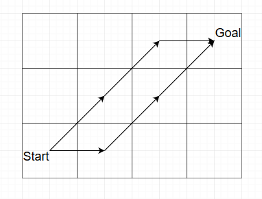
Here I want to walk on a grid from the bottom left to the top right. There are three equivalent short paths I could take, two of which are visualized here. In one I walk diagonally up-right, then up-right again, then right. In the other path I walk right first, then diagonally up-right, then up-right again. These two should have exactly the same cost, but whether they do or not depends on which constants you pick.

Let’s say we pick a cost of 1 to go north, east, west or south, and we pick a cost of 1.41 to go diagonally. (the real cost is sqrt(2), but 1.41 should be close enough) Then the first path adds up to 1.41 + 1.41 + 1 = 3.82, and the second path adds up to 1 + 1.41 + 1.41 = 3.82. Except since these are floating point numbers, they don’t add exactly to 3.82, and of course these two actually give slightly different results. The first one comes out to 3.8199999332427978515625, and the second comes out to 3.81999969482421875. Can you spot the difference? Computers certainly can. Now usually you would just say that this is why you don’t compare floats exactly. You always put in a little wiggle room. But as I said above, I have been bitten by that in the past because that can break in really subtle ways.

So how would we find numbers that add exactly in cases like this? The solution is to round the floats. But clearly rounding sqrt(2) to 1.41 didn’t work. So how would we round floating point numbers in a way that’s friendly to floating point math? For that we have to see how floating point numbers work. A floating point number consists of

• 1 sign bit
• 8 bits for the exponent
• 23 bits for the mantissa

The sign bit is clearly not interesting for us. So what about the exponent? When you increase the exponent on a number like 1.41, you get 2.82. When you decrease the exponent, you get 0.705. (except you never really get exactly these numbers) So we clearly don’t want to mess with the exponent when rounding floats. That leaves the mantissa. To illustrate how we’re going to round the mantissa, I’m going to print the 23 bits of the mantissa on the left, and the corresponding float value on the right. Starting with sqrt(2):

01101010000010011110011: 1.41421353816986083984375
01101010000010011110010: 1.4142134189605712890625
01101010000010011110000: 1.4142131805419921875
01101010000010011100000: 1.414211273193359375
01101010000010011000000: 1.41420745849609375
01101010000010010000000: 1.4141998291015625
01101010000010000000000: 1.4141845703125
01101010000000000000000: 1.4140625
01101000000000000000000: 1.40625
01100000000000000000000: 1.375
01000000000000000000000: 1.25
00000000000000000000000: 1

In each of these steps I changed a 1 to a 0. This rounds the number down. We could also round up, but rounding down is easier and we don’t really care which way we lose precision. So what we see here is how floating point numbers change as we round them to have more zero bits at the end.

And that gives us a bunch of floating point numbers that are going to guarantee associativity for a longer time. To test that I wrote a small simulation that randomly walks straight or diagonally on a grid, and adds up the cost. For the first number, I very quickly found paths like in my picture above where two paths with identical costs actually don’t end up with identical floating point numbers. In fact I could also do it in just three steps, just like in the picture. For the third row I already needed 32 steps. For the fifth row I needed 128 steps, for the seventh row I needed 2048 steps, and for the eighth row, I needed more than 100,000 steps on a grid before I lost associativity. Meaning if you use the number 1.4140625 as a constant for doing diagonal steps, you can have grids with a diameter of 100,000 cells before two paths that should have identical cost will ever show up as having different costs. Which is good enough for me.

So my recommendation is that you use 1.4140625, then you can compare your floats directly without needing to use any wiggle room.

How do we find numbers like this? Here is small chunk of C++ code that sets one bit at a time to zero:

union FloatUnion
{
    float f;
    struct
    {
        unsigned mantissa : 23;
        unsigned exponent : 8;
        unsigned sign : 1;
    };
};

void TruncateFloat(float to_print)
{
    FloatUnion f = { to_print };
    std::cout << f.f << std::endl;
    for (int bit = 0; bit < 23; ++bit)
    {
        f.mantissa = f.mantissa & ~(1 << bit);
        std::cout << f.f << std::endl;
    }
}

Feel free to use this code however you like. (MIT license, copyright 2018 Malte Skarupke)

So how do we use this to speed up A* path finding?

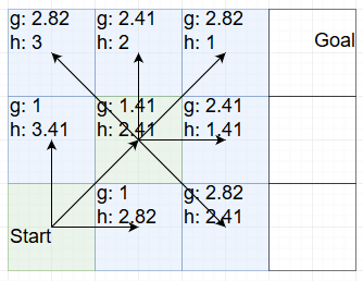
The idea isn’t mine, I have it from Steve Rabin. But these rounded floating point numbers make it easier. Before we get there, I have to walk through one run of A* to explain how it works. (because I can’t assume that you know A*) In A* you keep track of two numbers for each node: 1. How long it took you to get to that node (usually called g) and 2. An estimate for how large the distance between the current node and the goal is. (usually called h) Then when we decide on which node to explore next, we pick the one where g+h is the smallest number. So for example let’s say we start A* and after looking at all the neighbors of the start node, we have this state:

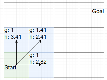
In this picture I made the start node green because we’re already finished with it. The blue nodes are the nodes that we consider next. The top left node has a total value of 1+3.41 = 4.41. The other two nodes have a total value of 1.41+2.41=1+2.82=3.82. The g distance is the distance from the start to this node, the h distance is the estimated distance to the goal. Since there are no obstacles in the way on this grid, the h value is actually always the real distance to the goal. But that won’t matter for this example. (oh and I’m using Steve Rabin’s Octile heuristic to compute the h value)

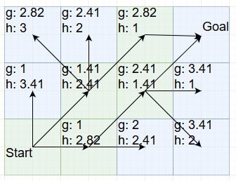
What this means is that when exploring the next node, both of the nodes on the right are equally good choices because they have the same value. So let’s explore the one at the bottom:

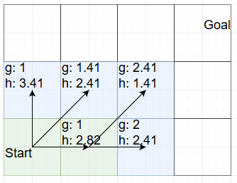
That gives us one new node with a bad total value (4.41) and one new node with a good total value (3.82) so we can choose between the two upper right values. I will expand the one on the left:

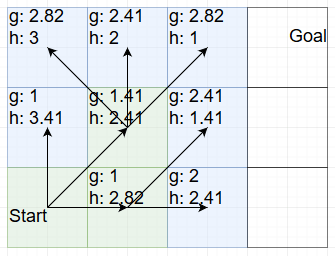
Once again we have two choices with a total value of 3.82. I will expand the top one:

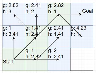
With that we have the goal within reach. We can’t end the search here though, because we have hit exactly the example that I started the blog post with: The path we chose rounds off to a slightly higher cost than the other path. So we also have to explore that one:

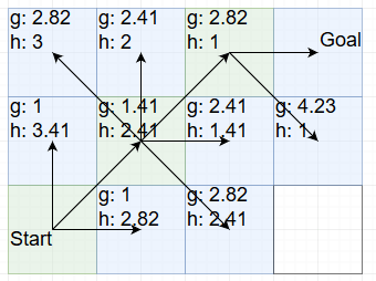
And with that we have now found the shortest path to the goal: Walk right, then walk diagonally up-right twice. It’s ever so slightly shorter than going diagonally up-right twice and then going right.

Having exact floating point math would allow us to skip that last step, but it would also allow another optimization:

When choosing between two nodes that have the same total value, explore the one with a larger g value first.

That trick speeds A* up a lot when walking across open terrain. Let’s go through it again, using this trick now:

We’re back at the start and we have two equal choices: Right and top-right both add up to 3.82. But top-right has a larger g value, so we choose that one:

Now we have three possible choices that add up to 3.82. Once again we choose the one with the largest g value and go top-right again:

And with that we’re at the goal. And we don’t need to explore any alternatives because they all have the same values. We simply walked straight there. The previous search had to explore 6 nodes, (including the goal) this one only had to explore 4. On bigger grids the difference gets bigger.

The trick of “among equal choices, prefer higher g” makes the A* path finding walk directly across open fields. And we don’t lose any correctness. If there is an obstacle in the way it will still explore the other paths that add up to the same number.

It’s a great trick. And it’s made easier by having floating point numbers that don’t have rounding errors when added. So choose 1.4140625 for diagonal steps. And if you’re using the octile heuristic, choose 0.4140625 for the constant in there. With those two numbers your grid would have to be more than 100,000 cells in width or height before you would ever get different costs for nodes that should have the same cost. So all equally good cells will actually have the exact same float representation.

Also if you can come up with other use cases for rounding floating point numbers like this, I would be curious to hear about them.