Probably Dance

edit: turns out you can get an even faster hash table by using this allocator with boost::multi_index. I now recommend that solution over the hash table from the post below. But anyway here is the original post:

This is a follow up post to “I Wrote a Fast Hash Table.”

And I’ll start off with a download link.

I’ve spent some time optimizing my sherwood_map implementation and now it is faster than boost::unordered_map and boost::multi_index. Which is what I would have expected from my first implementation, but it turns out that those containers are pretty damn fast.

If you don’t know what Robin Hood Linear Probing is I would encourage you to read the previous post and the post that I linked to from that one. With that said let’s talk about details.

The crucial optimization for speeding up my hash table was to store some information about each bucket.

The problem with Robin Hood Linear Probing is that you may have to search many buckets until you know whether or not your element is in the map. And my initial implementation was slow because I had to do an integer division to figure out when to stop iterating. But because of the way that Robin Hood hashing works, you can be sure that all elements of a bucket are stored next to each other. I’m not quite sure how to prove this, but here’s an attempt at an explanation: If you’re iterating over the array in the table and you come across an element which is from a different bucket, there are two cases: A) the element comes from a bucket in front of your bucket. In that case you will never take its position because its distance to its initial bucket will be larger than your distance to your initial bucket, and you don’t steal from the poor. B) the element comes from a bucket behind your bucket. In that case you will always take its position because its distance to its initial bucket will be less than your distance to your initial bucket. If you repeat those two situations many times all elements from the same bucket will be bunched together.

Because of that I store two additional pieces of information about each bucket: 1) the number of elements in that bucket, and 2) the distance in the array from the bucket to the first element in the bucket. With that information I only have to find the bucket of an element and then know exactly which elements in the array I have to look at.

One concern with Robin Hood Linear Probing is that if you store large elements in your hash table, the table would slow down because those large elements will always push the next element into a new cache line. A potential solution for this is to use two arrays for storage: One to store the hashes and the metadata, and one to store key/value pairs. That way you can iterate over the hash array quickly, and you only have to look into the key/value array when you find a matching hash. The sherwood_map implementation from my last post was written with that optimization.

Unfortunately that optimization made successful lookups slow because you had to look at two arrays, thus getting two cache misses. Since I consider lookups to be the most important operation of a map, I decided to only use one array for the implementation that I ship with this blog post.

I have included both versions in my profiling code though. fat_sherwood_map has two arrays, thin_sherwood_map stores everything in one array.

I’ve also tried using using powers of two for the map size instead of prime numbers. This allows you to do a faster lookup because you don’t have to do an integer division when finding the initial bucket. Had I included that implementation in the graphs below, it would easily have beaten all other implementations. Unfortunately it is very easy to come up with situations where a power of two sized map is slower. For example when using 16 byte aligned pointers as keys. If you know that you will never do that and that you have a good hashing function that gives you few bucket conflicts, then using a power of two sized map is much faster than using prime numbers. I don’t use that implementation though because it can not be generally used.

Let’s get to performance measurements. Which means pretty graphs. I have used the code from Joaquín M López Muñoz’ blog to profile the hash table against std::unordered_map (from libstdc++), boost::unordered_map and boost::multi_index. I compiled my code using GCC 4.8.2. I don’t provide graphs for other compilers because these take literally all day to generate.

I have run each test once with a small, medium and large values. The small value is just an int, the medium value is an int and two strings, and the large value is an int followed by a 1024 byte array. I always use an int as the key.

	Small	Medium	Large
Insert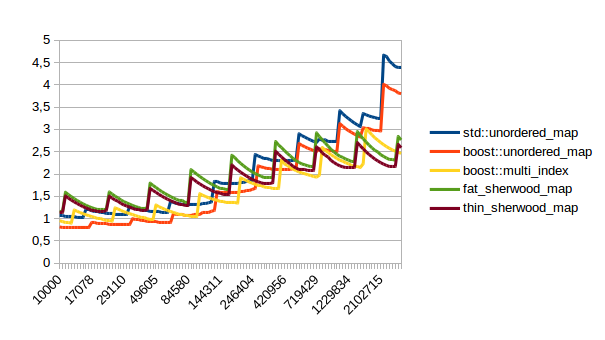
Reserve then Insert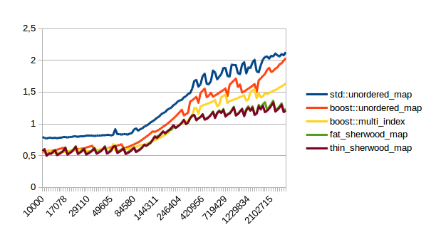
Erase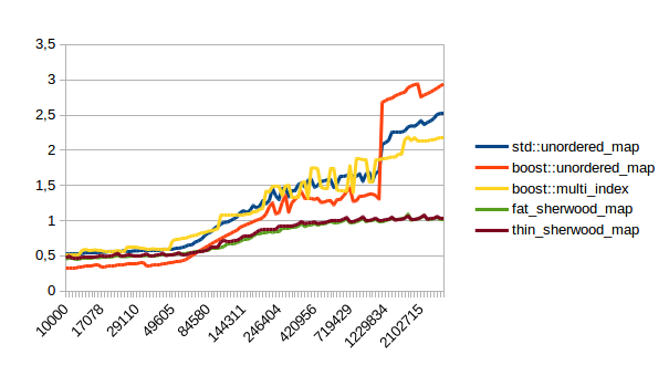
Successful Lookup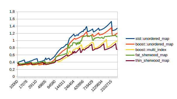
Unsuccessful Lookup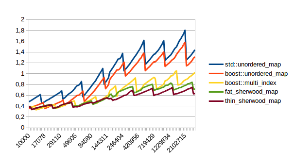

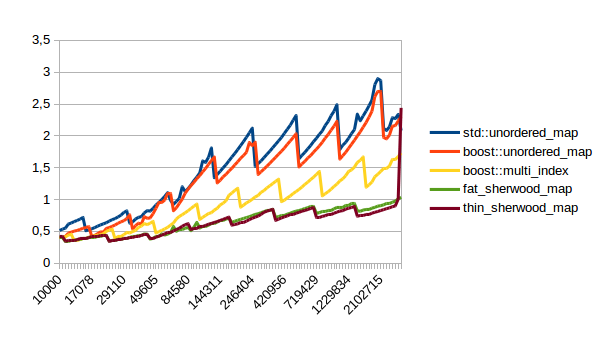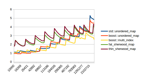
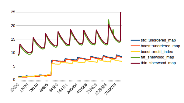
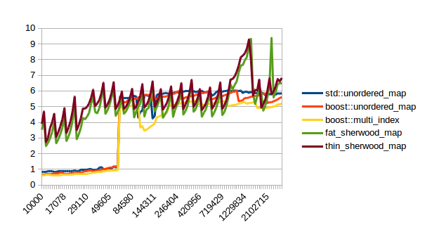
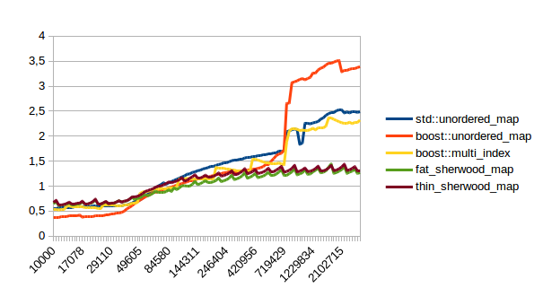
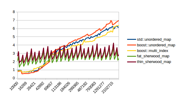
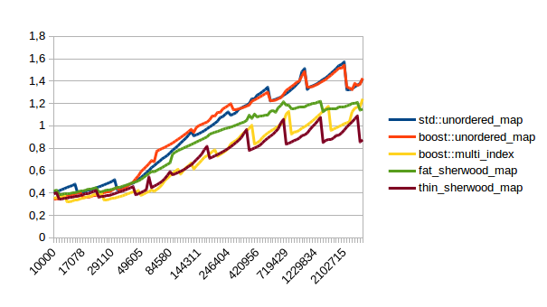
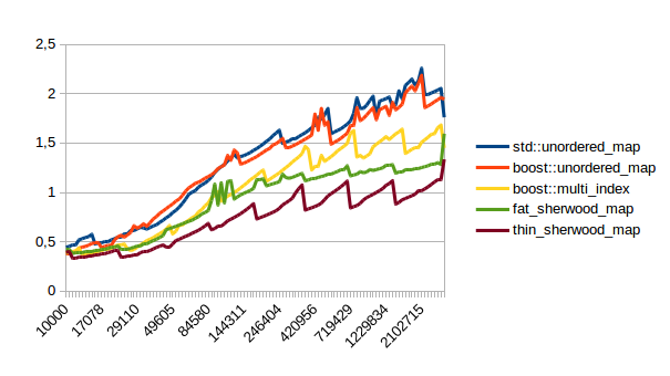
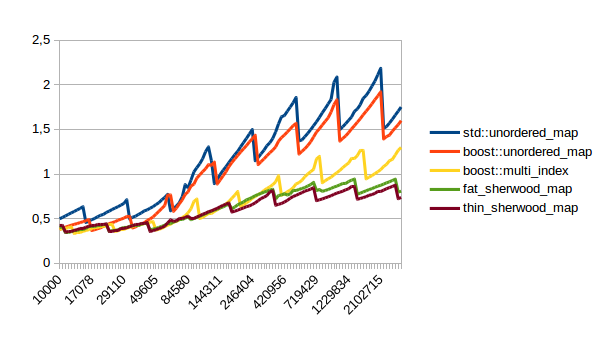
In all of these thin_sherwood_map is the sherwood_map implementation that I uploaded with this post, so the brown line is the one you want to be looking at. You can click on the images to get bigger pictures.

The X axis is the number of elements in the map, the Y axis is a somewhat arbitrary performance metric where smaller numbers are better.

In general this is what I expected, with one exception: I have no idea why sherwood_map does better in lookups when the value sizes are bigger. I would have expected it to do worse for large values.

There are many weird spikes in these graphs that could probably be investigated to figure out why the performance of certain maps sometimes changes drastically. One spike that I can explain is the one at the end of the insert graph for sherwood_map for large elements: I simply ran out of memory. Turns out the OS doesn’t like it if you want several gigabytes of contiguous memory.

I’m kind of disappointed that all graphs flatten out to the left hand side. It seems like all maps are equally fast for small number of elements. I believe that that’s the cost of doing an integer division followed by a pointer dereference, which is the constant cost that all of these hash tables have in common. A power of two sized map (which doesn’t need the integer division) beats the other maps on the left hand side.

So when should you use sherwood_map over unorederd_map or boost::multi_index? From the graphs above I would say you should use sherwood_map either when you plan to perform many lookups, (which is probably the usual use case for using a hash table) or when your values are somewhat small and you can call reserve() on the map.

You should use another implementation if

• You have large values and plan to modify the map a lot
• You need iterators or references to remain valid after inserts and erases.
• You can’t offer noexcept move assignment and construction.
• You need custom allocator propagation. I don’t support that feature yet, sorry.

The two main things I’ve learned from this are 1. The standard containers are pretty damn fast already and are difficult to beat. If you have your own hash table implementation I would encourage you to measure it against std::unordered_map. You are probably no faster or even slower. 2. It takes ages to implement a fast container with an interface that’s as flexible as the STL interface. This container didn’t follow the 80/20 rule and behaved more like the 95/5 rule. I spent 95% of my time on the last 5%.

And once again here’s the download link.