I Wrote The Fastest Hashtable
by Malte Skarupke
I had to get there eventually. I had a blog post called “I Wrote a Fast Hashtable” and another blog post called “I Wrote a Faster Hashtable.” Now I finally wrote the fastest hashtable. And by that I mean that I have the fastest lookups of any hashtable I could find, while my inserts and erases are also really fast. (but not the fastest)
The trick is to use Robin Hood hashing with an upper limit on the number of probes. If an element has to be more than X positions away from its ideal position, you grow the table and hope that with a bigger table every element can be close to where it wants to be. Turns out that this works really well. X can be relatively small which allows some nice optimizations for the inner loop of a hashtable lookup.
If you just want to try it, here is a download link. Or scroll down to the bottom of the blog post to the section “Source Code and Usage.” If you want more details read on.
Type of Hashtable
There are many types of hashtables. For this one I chose
- Open addressing
- Linear probing
- Robing hood hashing
- Prime number amount of slots (but I provide an option for using powers of two)
- With an upper limit on the probe count
I believe that the last of these points is a new contribution to the world of hashtables. This is the main source of my speed up, but first I need to talk about all the other points.
Open addressing means that the underlying storage of the hashtable is a contiguous array. This is not how std::unordered_map works, which stores every element in a separate heap allocation.
Linear probing means that if you try to insert an element into the array and the current slot is already full, you just try the next slot over. If that one is also full, you pick the slot next to that etc. There are known problems with this simple approach, but I believe that putting an upper limit on the probe count resolves that.
Robin Hood hashing means that when you’re doing linear probing, you try to position every element such that it is as close as possible to its ideal position. You do this by moving objects around whenever you insert or erase an element, and the method for doing that is that you take from rich elements and give to poor elements. (hence the name Robin Hood hashing) A “rich” element is an element that received a slot close to its ideal insertion point. A “poor” element is one that’s far from its ideal insert point. When you insert a new element using linear probing you count how far you are from your ideal position. If you are further from your ideal position than the current element, you swap the new element with the existing element and try to find a new spot for the existing element.
The prime number amount of slots means that the underlying array has a prime number size. Meaning it grows for example from 5 slots to 11 slots to 23 slots to 47 slots etc. Then to find the insertion point you simply use the modulo operator to assign the hash value of an element to a slot. The other most common choice is to use powers of two to size your array. Later in this blog post I will go more into why I chose prime numbers by default and when you want to use which.
A Upper Limit for the Probe Count
With the basics out of the way, let’s talk about my new contribution: Limiting how many slots the table will look at before it gives up and grows the underlying array.
My first idea was to set this to a very low number, say 4. Meaning when inserting I try the ideal slot and if that doesn’t work I try the next slot over, the next slot over, the slot after that and if all of them are full I grow the table and try inserting again. This works great for small tables, but when I insert random values into a large table, I would get unlucky all the time and hit four probes and I would have to grow the table even though it was mostly empty.
Instead I found that using log2(n) as the limit, where n is the number of slots in the table, makes it so that the table only has to reallocate once it’s roughly two thirds full. That is when inserting random values. When inserting sequential values the table can be filled up completely before it needs to reallocate.
Even though I found that the table can fill up to roughly two thirds, every now and then it would have to reallocate when it’s only 60% full. Or rarely even when it’s only 55% full. So I set the max_load_factor of the table to 0.5. Meaning the table will grow when its half full, even when it hasn’t reached the limit of the probe count. The reason for that is that I want a table that you can trust to reallocate only when you actually grow it: If you insert a thousand elements, then erase a couple elements and then insert that same number of elements again, you can be almost certain that the table won’t reallocate. I can’t put a number on the certainty, but I ran a simple test where I built thousands of tables of all kinds of sizes and filled them with random integers. Overall I inserted hundreds of billions of integers into the tables, and they only reallocated at a load factor of less than 0.5 once. (that time the table grew when it was 48% full, so it grew slightly too soon) So I think you can trust that this will very, very rarely reallocate when you weren’t expecting it.
That being said if you don’t need control over when the table grows, feel free to set the max_load_factor higher. It’s totally safe to set it to 0.9: Robin hood hashing combined with the maximum probe count will ensure that all operations remain fast. Don’t set it to 1.0 though: You can get into bad situations when inserting then because you might hit a case where every single element in the table has to be shifted around when inserting the last element. (say every element is in the slot it wants to be, except the very last slot is empty. Then you insert an element that wants to be in the first slot, but the first slot is already full. So it will go into the second slot, pushing the second element one over, which will push the third element one over etc. all the way through the table until the element in the second to last slot gets pushed into the last slot. You now have a table where every element except for the first is one slot from its ideal slot so lookups are still really fast, but that last insert took a long time) By keeping a few empty slots around you can ensure that newly inserted elements only have to move a few elements over until one of them finds an empty slot.
So if I set the max_load_factor so low that I never reach the probe count limit anyway, why have the limit at all? Because it allows a really neat optimization: Let’s say you rehash the table to have 1000 slots. My hashtable will then grow to 1009 slots because that’s the closest prime number. The log2 of that is 10, so I set the probe count limit to 10. The trick now is that instead of allocating an array of 1009 slots, I actually allocate an array of 1019 slots. But all other hash operations will still pretend that I only have 1009 slots. Now if two elements hash to index 1008, I can just go over the end and insert at index 1009. I never have to do any bounds checking because the probe count limit ensures that I will never go beyond index 1018. If I ever have eleven elements that want to go into the last slot, the table will grow and all those elements will hash to different slots. Without bounds checking, my inner loops are tiny. Here is what the find function looks like:
iterator find(const FindKey & key)
{
    size_t index = hash_policy.index_for_hash(hash_object(key));
    EntryPointer it = entries + index;
    for (int8_t distance = 0;; ++distance, ++it)
    {
        if (it->distance_from_desired < distance)
            return end();
        else if (compares_equal(key, it->value))
            return { it };
    }
}
It’s basically a linear search. The assembly of this code is beautiful. This is better than simple linear probing in two ways: 1. No bounds checking. Empty slots have -1 in their distance_from_desired value so the empty case is the same case as finding a different element. 2. This will do at most log2(n) iterations through the loop. Normally the worst case for looking things up in a hashtable is O(n). For me it’s O(log n). This makes a real difference. Especially since linear probing actually makes it pretty likely that you will hit the worst case since linear probing tends to bunch elements together.
My memory overhead on this is one byte per element. I store the distance_from_desired in an int8_t. That being said that one byte will be padded out to the alignment of the type that you insert. So if you insert ints, the one byte will get three bytes of padding so there is four bytes of overhead per element. If you insert pointers there will be 7 bytes of padding so you get eight bytes of overhead per element. I’ve thought about changing my memory layout to solve this, but my worry is that then I would have two cache misses for each lookup instead of one cache miss. So the memory overhead is one byte per element plus padding. Oh and with a max_load_factor of 0.5 (which is the default) your table will only be between 25% and 50% full, so there is more overhead there. (but once again it’s safe to increase the max_load_factor to 0.9 to save memory while only suffering a small decrease in speed)
Lookup Performance
Measuring hash tables is actually not easy. You need to measure at least these cases:
- Looking up an element that’s in the table
- Looking up an element that can not be found in the table
- Inserting a bunch of random numbers
- Inserting a bunch of random numbers after calling reserve()
- Erasing elements
And you need to run each of these with different keys and different sizes of values. I use an int or a string as the key, and I use value types of size 4, 32 and 1024. I will prefer to use int keys because with strings you’re mostly measuring the overhead of the hash function and the comparison operator, and that overhead is the same for all hash tables.
The reason for testing both successful lookups and unsuccessful lookups is that for some tables there is a huge difference in performance between these cases. For example I came across a really bad case when inserting all the numbers from 0 to 500000 into a google::dense_hash_map (meaning they were not random numbers) and then did unsuccessful lookups: The hashtable suddenly was five hundred times slower than it usually is. This is a edge case of using a power of two for the size of the table. I’ll go more into when you should pick powers of two and when you should pick prime numbers below. This example suggests that maybe I should measure each of these with random numbers and with sequential numbers, but that ended up being too many graphs. So I will only test tables with random numbers which should prevent bad cases caused by specific patterns.
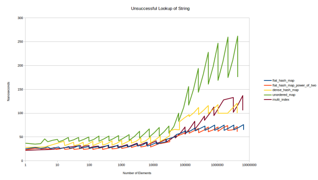
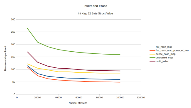
The first graph is looking up an element that’s in the table:
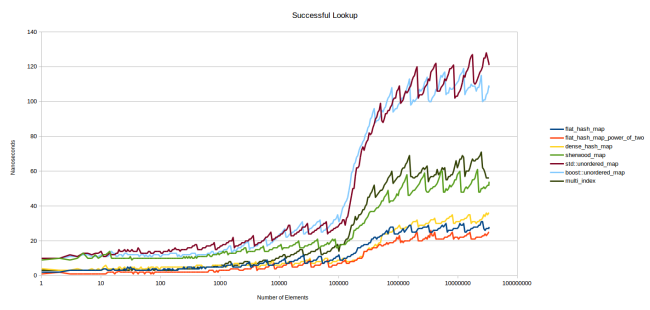
This is a pretty dense graph so let’s spend some time on this one. flat_hash_map is the new hash table I’m presenting in this blog post. flat_hash_map_power_of_two is that same hash table but using powers of two for the array size instead of prime numbers. You can see that it’s much faster and I’ll explain why that is below. dense_hash_map is google::dense_hash_map which is the fastest hashtable I could find. sherwood_map is my old hashtable from my “I Wrote a Faster Hashtable” blog post. It’s embarrassingly slow… std::unordered_map and boost::unordered_map are self-explanatory. multi_index is boost::multi_index.
I want to talk about this graph a little. The Y-axis is the number of nanosecons that it takes to look up a single item. I use google benchmark and that calls table.find() over and over again for half a second, and then counts how many times it was able to call that function. You get nanoseconds by dividing the time that all iterations took together by the loop count. All the keys I’m looking for are guaranteed to be in the table. I chose to use a log scale for the X axis because performance tends to change on a log scale. Also this makes it possible to see the performance at different scales: If you care about small tables, you can look at the left side of the graph.
The first thing to notice is that all of the graphs are spiky. This is because all hashtables have different performance depending on the current load factor. Meaning depending on how full they are. When a table is 25% full lookups will be faster than when it’s 50% full. The reason for this is that there are more hash collisions when the table is more full. So you can see the cost go up until at some point the table decides that it’s too full and that it should reallocate, which makes lookups fast again.
This would be very clear if I were to plot the load factors of each of these tables. One more thing that would be clear is that the tables at the bottom have a max_load_factor of 0.5, the tables at the top have a max_load_factor of 1.0. This immediately raises the question of “wouldn’t those other tables also be faster if they used a max_load_factor of 0.5?” The answer is that they would only be a little faster, but I will answer that question more fully with a different graph further down. (but just from the graph above you can see that the lowest point of the upper graph, when those tables have just reallocated and have a load factor of just over 0.5 is far over the highest point of the lower graphs, just before they reallocate because their load factor is just under 0.5)
Another thing that we notice is that all the graphs are essentially flat on the left half of the screen. This is because the table fits entirely into the cache. Only when we get to the point where the data doesn’t fit into my L3 cache do we see the different graphs really diverge. I think this is a big problem. I think the numbers on the right are far more realistic than the numbers on the left. You will only get the numbers on the left if the element you’re looking for is already in the cache.
So I tried to come up with a test that would measure how fast the table would be if it wasn’t in the cache: I create enough tables so that they don’t all fit into L3 cache and I use a different table for every element that I look up. Let’s say I want to measure a table that has 32 elements in it and the elements in the table are 8 bytes in size. My L3 cache is 6 mebibytes so I can fit roughly 25000 of these tables into my L3 cache. To be sure that the tables won’t be in the cache I actually create three times that number, meaning 75000 tables. And each lookup is from a different table. That gives me this graph:

First, I removed a couple of the lines because they didn’t add much information. boost::unordered_map is usually the same speed as std::unordered_map (sometimes it’s a little faster, but it’s still always above everything else) and nobody cares about my old slow hash table sherwood_map. So now we’re left with just the important ones: std::unordered_map as a normal node based container, boost::multi_index as a really fast node based container, (I believe that std::unordered_map could be this fast) google::dense_hash_map as a fast open addressing container, and my new container in its prime number version and its power of two version.
So in this new benchmark, where I try to force a cache miss, we can see big differences very early on. What we find is that the pattern that we saw at the end of the last graph emerges very early in this graph: Starting at ten elements in the table there are clear winners in terms of performance. This is actually pretty impressive: All of these hash tables maintain consistent performance across many different orders of magnitude.
Let’s also look at the graph for unsuccessful lookups: Meaning trying to find an item that is not in the table:

When it comes to unsuccessful lookups the graph is even more spiky: The load factor really matters here. The more full a table is the more elements the search has to look at before it can conclude that an item is not in the table. But I’m actually really happy about how my new table is doing here: Limiting the probe count seems to work. I get more consistent performance than any other table.
What I take from these graphs is that my new table is a really big improvement: The red line, with the powers of two, is my table configured the same way as dense_hash_map: With max_load_factor 0.5 and using a power of two to size the table so that a hash can be mapped to a slot just by looking at the lower bits. The only big difference is that my table requires one byte of extra storage (plus padding) per slot in the table. So my table will use slightly more memory than dense_hash_map.
The surprising thing is that my table is as fast as dense_hash_map even when using prime numbers to size the table. So let me talk about that.
Prime Numbers or Powers of Two
There are three expensive steps in looking up an item in a hashtable:
- Hashing the key
- Mapping the key to a slot
- Fetching the memory for that slot
Step 1 can be really cheap if your key is an integer: You just cast the int to a size_t. But this step can be more expensive for other types, like strings.
Step 2 is just an integer modulo.
Step 3 is a pointer dereference, for std::unordered_map it’s actually multiple pointer dereferences.
Intuitively you would expect that if you don’t have a very slow hash function, step 3 is the most expensive of these three. But if you’re not getting cache misses for every single lookup, chances are that the integer modulo will end up being your most expensive operation. Integer modulo is really slow, even on modern hardware. The Intel manual lists it as taking between 80 and 95 cycles.
This is the main reason why really fast hash tables usually use powers of two for the size of the array. Then all you have to do is mask off the upper bits, which you can do in one cycle.
There is however one big problem with using a power of two: There are many patterns of input data that result in lots of hash collisions when using powers of two. For example here is that last graph again, except I didn’t use random numbers:
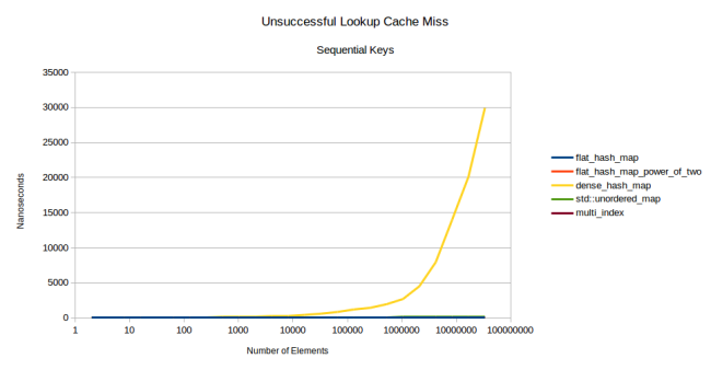
Yes you see correctly that google::dense_hash_map just takes off into the stratosphere. What pattern of inputs did I have to use to get such poor performance out of dense_hash_map? It’s just sequential numbers. Meaning I insert all numbers [0, 1, 2, …, n – 2, n – 1]. If you do that, trying to look up a key that’s not in the table will be super slow. Successful lookups will still be fine. But if some of your lookups are for keys that are in the table and some are for keys that are not, then you might find that some of your lookups are a thousand times slower than others.
Another example of bad performance due to using powers of two is how the standard hashtable in Rust was accidentally quadratic when inserting keys from one table into another. So using powers of two can bite you in non-obvious ways.
It just so happens that my hashtable doesn’t suffer from either of these problems: The limit of the probe count resolves both of these problems in the best way possible. The table doesn’t even have to reallocate unnecessarily. Does that mean that I’m immune against problems that come from using powers of two? No. For example one problem that I have personally experienced in the past is that when you insert pointers into a hash table that uses powers of two, some slots will never be used. The reason is heap allocations in my program were sixteen byte aligned and I used a hash function that just reinterpret_casted the pointer to a size_t. Because of that only one out of sixteen slots in my table was ever used. You would run into the same problem if you use the power of two version of my new hashtable.
All of these problems are solvable if you’re careful about choosing a hash function that’s appropriate for your inputs. But that’s not a good user experience: You now always have to be vigilant when using hashtables. Sometimes that’s OK, but sometimes you just want to not have to think too much about this. You just want something that works and doesn’t randomly get slow. That’s why I decided to make my hashtable use prime number sizes by default and to only give an option for using powers of two.
Why do prime numbers help? I can’t quite explain the math behind that, but the intuition is that since the prime number doesn’t share common divisors with anything, all numbers get different remainders. For example let’s say I’m using powers of two, my hashtable has 32 slots, and I am trying to insert pointers which are all sixteen byte aligned. (meaning all my numbers are multiples of sixteen) Now using integer modulo to find a slot in the table will only ever give me two possible slots: slot 0 or slot 16. Since 32 is divisible by 16, you simply can’t get more possible values than that. If I use a prime numbered size instead I don’t run into that problem. For example if I use the prime number 37, then all divisions using multiples of sixteen give me different slots in the table, and I will use all 37 slots. (try doing the math and you will see that the first 37 multiples of 16 all would end up in different slots)
So then how do we solve the problem of the slow integer modulo? For this I’m using a trick that I copied from boost::multi_index: I make all integer modulos use a compile time constant. I don’t allow all possible prime numbers as sizes for the table. Instead I have a selection of pre-picked prime numbers and will always grow the table to the next largest one out of that list. Then I store the index of the number that your table has. When it later comes time to do the integer modulo to assign the hash value to a slot, you will see that my code does this:
switch(prime_index)
{
case 0:
    return 0llu;
case 1:
    return hash % 2llu;
case 2:
    return hash % 3llu;
case 3:
    return hash % 5llu;
case 4:
    return hash % 7llu;
case 5:
    return hash % 11llu;
case 6:
    return hash % 13llu;
case 7:
    return hash % 17llu;
case 8:
    return hash % 23llu;
case 9:
    return hash % 29llu;
case 10:
    return hash % 37llu;
case 11:
    return hash % 47llu;
case 12:
    return hash % 59llu;
//
// ... more cases
//
case 185:
    return hash % 14480561146010017169llu;
case 186:
    return hash % 18446744073709551557llu;
}
Each of these cases is a integer modulo by a compile time constant. Why is this a win? Turns out if you do a modulo by a constant, the compiler knows a bunch of tricks to make this fast. You get custom assembly for each of these cases and that custom assembly will be much faster than an integer modulo would be. It looks kinda crazy but it’s a huge speed up.
You can see the difference in the graphs above: Using prime numbers is a little bit slower, but it’s still really fast when compared to other hash tables, and you’re immune against most bad cases of hash tables. Of course you’re never immune against all bad cases. If you really worry about that, you should use std::map with its strict upper bounds. But the difference is that when using powers of two, there are many bad cases and you have to be careful not to stumble into them. When using prime numbers you will basically only hit a bad case if you intentionally create bad keys.
That brings up security: A clever attack that you can do on hash tables is that you insert keys that all collide with each other. How might you do that? If you know that a website uses a hashtable in its internal caches, then you could engineer website requests such that all your requests will collide in that hashtable. Like that you can really slow down the internal cache of a webserver and possibly bring down the website. So for example if you know that google uses dense_hash_map internally and you see the graph above where it gets really slow if you insert sequential numbers, you could just request sequential websites and hope that that pollutes their cache. You might think that setting an upper limit on the probe count prevents attackers from filling up your table with bad keys. That is true: My hashtable will not suffer from this problem. However a new attack immediately presents itself: If you know which prime numbers I use internally you could insert keys in an order so that my table repeatedly hits the limit of the probe count and has to repeatedly reallocate. So the new attack is that you can make the server run out of memory. You can solve this by using a custom hash function, but I can’t give you advice for what such a hash function should look like. All I can tell you is that if you use the hashtable in an environment where users can insert keys, don’t use std::hash as your hash function and use something stateful instead that can’t be predicted ahead of time. On the other hand if you don’t think that people will be malicious, you can be confident that using the prime number version of my hashtable will result in an even spread of values and there will be no problems.
But let’s say you know that your hash function returns numbers that are well distributed and that you’re rarely going to get hash collisions even if you use powers of two. Then you should use the power of two version of my table. To do that you have to typedef a hash_policy in your hash function object. I decided to put this customization point into the hash function object because that is the place that actually knows the quality of the returned keys.
So you put this typedef into your custom hash function object:
struct CustomHashFunction
{
    size_t operator()(const YourStruct & foo)
    {
        // your hash function here
    }
    typedef ska::power_of_two_hash_policy hash_policy;
};

// later:
ska::flat_hash_map<YourStruct, int, CustomHashFunction> your_hash_map;
In your custom hash function you typedef ska::power_of_two_hash_policy as hash_policy. Then my flat_hash_map will switch to using powers of two. Also if you know that std::hash is good enough in your case, I provide a type called power_of_two_std_hash that will just call std::hash but will use the power_of_two_hash_policy:
ska::flat_hash_map<K, V, ska::power_of_two_std_hash<K>> your_hash_map;
With either of these you can get a faster hashtable if you know that you won’t be getting too many hash collisions.
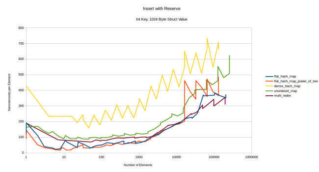
Insert and Erase Performance
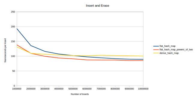
After that lengthy detour of talking about hash table theory let’s get back to the performance of my table. Here is a graph that measures how long it takes to insert an item into a map. The way I measure this is that I measure how long it takes to insert N elements, then I divide the time by N to get the time that the average element took. The first graph is the speed if I do not call reserve() before inserting:

This graph is also spiky, but the spikes point in the other direction. Any time that the table has to reallocate the average cost shoots up. Then that cost gets amortized until the table has to reallocate again.
The other point about this graph is that on the left half you once again only have tables that fit entirely in the L3 cache. I decided to not write a cache-miss-triggering test for this one because that would take time and we learned above that just looking at the right half is a good approximation for a cache miss.
Here google::dense_hash_map beats my new hash table, but not by much. My table is still very fast, just not quite as fast as dense_hash_map. The reason for this is that dense_hash_map doesn’t move elements around when inserting. It simply looks for an empty slot and inserts the element. The Robin Hood hashing that I’m using requires that I move elements around when inserting to keep the property that every node is as close to its ideal position as possible. It’s a trade-off where insertion becomes more expensive, but lookups will be faster. But I’m happy with how it seems to only have a small impact.
Next is the time it takes to insert elements if the table had reserve() called ahead of time:

I don’t know what’s happening with the node-based containers at the end there. It might be fun to investigate what’s going on there, but I didn’t do that. I actually have a suspicion that that’s due to the malloc call in my standard library. (Linux gcc) I had several problems with it while measuring this graph and others because some operations would randomly take a long time.
But overall this graph looks similar to the last one, except less spiky because the reserve removes the need for reallocations. I have fast inserts, but they’re not as fast as those of google::dense_hash_map.
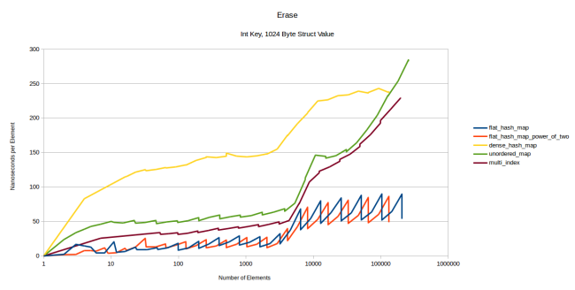
Finally let’s look at how long it takes to erase elements. For this I built a map of N elements, then measured how long it takes to erase every element in the map in a random order. Then I would divide the time it takes to erase all elements by N to get the cost per element:

The node based containers are slow once again, and the flat containers are all roughly equally fast. dense_hash_map is slightly faster than my hash table, but not by much: It takes roughly 20 nanoseconds to erase something from dense_hash_map and it takes roughly 23 nanoseconds to erase something from my hash table. Overall these are both very fast.
But there is one big difference between my table and dense_hash_map: When dense_hash_map erases an element, it leaves behind a tombstone in the table. That tombstone will only be removed if you insert a new element in that slot. A tombstone is a requirement of the quadratic probing that google::dense_hash_map does on lookup: When an element gets erased, it’s very difficult to find another element to take its slot. In Robin Hood hashing with linear probing it’s trivial to find an element that should go into the now empty slot: just move the next element one forward if it isn’t already in its ideal slot. In quadratic probing it might have to be an element that’s four slots over. And when that one gets moved you have to again solve the problem of finding a node to insert into the newly vacated slot. So instead you insert a tombstone and then the table knows to ignore tombstones on lookup. And they will be replaced on the next insert.
What this means though is that the table will get slightly slower once you have tombstones in your table. So dense_hash_map has a fast erase at the cost of slowing down lookups after an erase. Measuring the impact of that is a bit difficult, but I believe I have found a test that works for this purpose: I insert and erase elements over and over again:
The way this test works is that I first generate a million random ints. Then I insert these into the hashtable and erase them again and insert them again. The trick is that I do this in a random order: So let’s say I only had the four integers 1, 2, 3 and 4. Then a valid order for “insert, erase and insert again” would be insert 1, insert 3, erase 1, insert 2, insert 4, erase 4, insert 4, insert 1, erase 2, erase 3, insert 3, insert 2. Every element gets inserted, erased and inserted again. But the order is random. The graph above counts the number of inserts and measures how long the insert takes per element. The first data point, all the way on the left is just inserting a million elements. The second data point is inserting a million elements, erasing them and inserting them again in a random order like I explained. The next data point does insert, erase, insert, erase, insert. So three inserts in total. You get the idea.
What we see is that at first dense_hash_map is faster because its inserts are faster. At the second data point my hashtable has already caught up to it. At the third data point my hashtable is winning, and at six million inserts even my prime number version is winning. The reason why my tables keep on getting faster is that as there are more erases, you would expect the average load factor of the table to go down. If you insert and erase a million items often enough, the table will always have close to 500,000 elements in it. So as you get further to the right in this graph, the table will be less full on average. My hash table can take advantage of that, but dense_hash_map has a bunch of tombstones in the table which prevent it from going faster. That being said if we compare dense_hash_map against other hash tables, it’s still very fast:

So from this angle it totally makes sense for dense_hash_map to use quadratic probing, even if that requires inserting tombstones into the table on erase. The table is still very fast, certainly much faster than any node based container. But the point remains that Robin Hood linear probing gives me a more elegant way of erasing elements because it’s easy to find which element should go into the empty slot. And if you have a table where you often erase and insert elements, that’s an advantage.
Comparing Tables with Different max_load_factor()
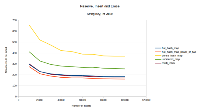
One final graph that I promised above is a way to resolve the problem that std::unordered_map and boost::multi_index use a max_load_factor of 1.0, while my table and google::dense_hash_map use 0.5. Wouldn’t the other tables also be faster if they used a lower max_load_factor? To determine that I ran the same benchmark that I used to generate the very first graph (successful lookups) but I set the max_load_factor to 0.5 on each table. And then I took measurements just before a table reallocates. I’ll explain it a bit better after the graph:
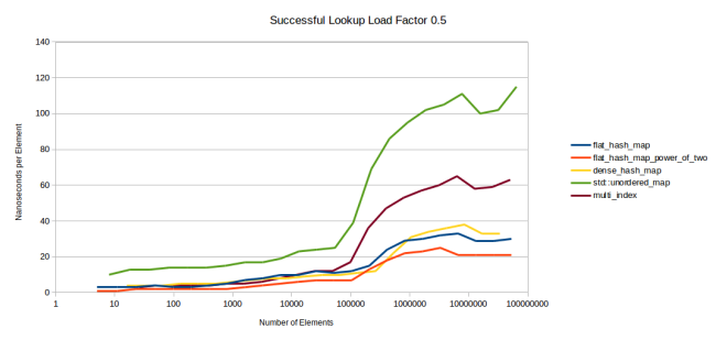
This is the same graph as the very first graph in this blog post, except all the tables use a max_load_factor of 0.5. And then I wanted to only measure these tables when they really do have the same load factor, so I measured each table just before it would reallocate its internal storage. So if you look back at the very first graph in this blog post, imagine that I drew lines from one peak to the next. If we want to directly compare performance of hashtables and we want to eradicate the effect of different hash tables using different max_load_factor values and different strategies for when they reallocate, I think this is the right graph.
In this graph we see that flat_hash_map is faster than dense_hash_map, just as it was in the initial graph. It’s now much clearer though because all the noisiness is gone. Btw that brief time where dense_hash_map is faster is a result of dense_hash_map using less memory: At that point dense_hash_map still fits in my L3 cache but my flat_hash_map does not. Knowing this I can also see the same thing in the first graph, but it’s much clearer here.
But the main point of this was to compare boost::multi_index and std::unordered_map, which use a max_load_factor of 1.0 to my flat_hash_map and dense_hash_map which use a max_load_factor of 0.5. As you can see even if we use the same max_load_factor for every table, the flat tables are faster.
This was expected, but I still think this was worth measuring. In a sense this is the truest measure of hash table performance because here all hash tables are configured the same way and have the same load factor: Every single data point has a current load factor of 0.5. That being said I did not use this method of measuring for my other graphs, because in the real world you probably will never change the max_load_factor. And in the real world you will see the spiky performance of the initial graph where similar tables can have very different performance, depending on how many hash collisions there are. (and the load factor is actually only one part of that, as I also discussed above when talking about powers of two vs prime numbers) And also this graph hides one benefit of my table: Limiting the probe count leads to more consistent performance, making the lines of my hash_map less spiky than the lines of other tables.
Different Keys and Values
So far every graph was measuring performance of a map from int to int. However there might be differences in performance when using different keys or larger values. First, here are the graphs for successful lookups and unsuccessful lookups when using strings as keys:

Yes, I went with the version of the graph where the table is already in the cache. It’s easier to generate. What we see here is that using a string is just moving all lines up a little. Which is expected, because the main cost here is that the hash function changed and the comparison is more expensive. Let’s look at unsuccessful lookups, too:
This is very interesting: It looks like looking for an element that’s not in the table is more expensive in google::dense_hash_map than in boost::multi_index. The reason for this is interesting: When creating a dense_hash_map you have to provide a special key that indicates that a slot is empty, and a special key that indicates that a slot is a tombstone. I used std::string(1, 0) and std::string(1, 255) respectively. But what this means is that the table has to do a string comparison to see that the slot is empty. All the other tables just do an integer comparison to see that a slot is empty.
That being said a string comparison that only compares a single character should be really cheap. And indeed the overhead is not that big. It just looks big above because every lookup is a cache hit. The cache miss picture looks different:

In this we can see that when the table is not already in the cache, dense_hash_map remains faster. Except it gets slower when the table gets very big. (more than a million entries) I didn’t find out why that is.
The next thing I tried to vary was the size of the value. What happens if I don’t have a map from an int to an int, but from an int to a 32 byte struct? Or from an int to a 1024 byte struct. So for the lookups I have 12 graphs in total ([int value, 32 byte value, 1024 byte value] x [int key, string key] x [successful lookup, unsuccessful lookup]) and most of them look exactly like the graphs above: All string lookups look the same independent of value size, and most int lookups also look the same. Except for one: Unsuccessful lookup of an int key and a 1024 byte value:
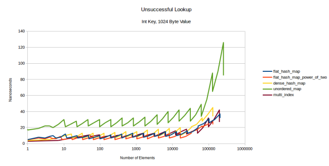
What we see here is that at a 1024 byte value, multi_index is actually competitive to the flat tables. The reason for this is that in an unsuccessful lookup you have to do the maximum number of probes, and with a value type that’s as huge as 1024 bytes, your prefetcher has to work hard. My table still seem to be winning, but for a value that’s this large, everything is essentially a node based container.
The reason why all other lookup graphs looked the same (and why I don’t show them) is this: For the node-based containers you don’t care how big the value is. Everything is a separate heap allocation anyway. For the flat containers you would expect that you would get more cache misses. But since the max_load_factor is 0.5, the element is usually found in the table pretty quickly. The most common case is exactly one lookup: Either you find it in the first probe or you know with the first probe that it won’t be in the table. Two probes also happen pretty often, but three probes are rare. Also at least in my table the lookups are just a linear search. CPUs are great at prefetching the next element in a linear search, no matter how big the item is.
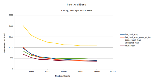
So lookups mostly don’t change with the size of the type, the graph for inserts and erases changes a lot though. Here is inserting with an int as a key and a 32 byte struct as a value:
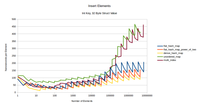
All the graphs have moved up a bit, but the graphs of the flat tables have moved up the most and have become more spiky: Reallocations hurt more when you have to move more data. The node based containers are not affected by this, and boost::multi_index stays competitive for a very long time. Let’s see what this looks like for a really large type, a 1024 byte struct:
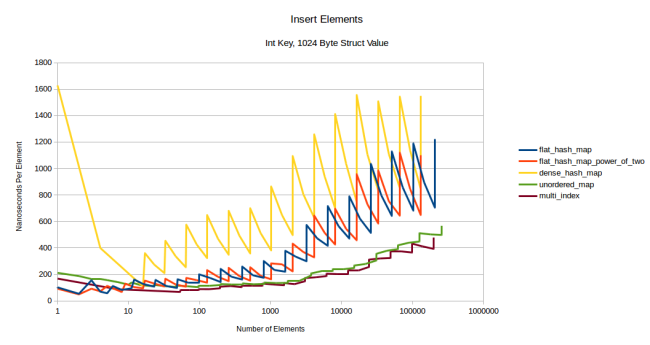
Now the order has flipped completely: The flat containers are more expensive and very spiky, the node based containers keep their speed. At this point reallocation cost dominates completely.
One oddity is that it’s really expensive to insert a single element into a dense_hash_map. (all the way on the left of the yellow line) The reason for this is that dense_hash_map allocates 32 slots at first and it fills all of them with a default constructed value type. Since my value type is 1024 bytes in size, it has to set 32 kib of data to 0. This probably won’t affect you, but I felt like I should explain the strange shape of the line.
The other thing that happened is that dense_hash_map is now slower than my hashtable. I didn’t look into why that is, but I would assume it’s for the same reason as the above paragraph: dense_hash_map fills every slot with a default constructed value type, so reallocation is even more expensive because all the slots have to be initialized, even the ones that will never be used.
If reallocation is expensive, the solution is to call reserve() on the container ahead of time so that no reallocation has to happen. Let’s see what happens when we insert the same elements but call reserve first:
When calling reserve first, my container is faster than the node based containers at first, but at some point boost::multi_index is still faster. dense_hash_map is still slower and again I think that’s because it initializes more elements than necessary and with a value this big, even just initializing the whole table to the “empty” key/value pair takes a lot of time. They could probably optimize this by only initializing the key to the “empty” key and not initializing the value, but then again how often do you insert a value that’s 1024 bytes? It’s neat as a benchmark to test the behavior of containers as the stored values grow very large, but it might not happen in the real world.
My containers are faster until they get large: at exactly 16385 elements there is a sudden jump in the cost. At 16384 elements things are still at the normal speed. Since every element in the container is 1028 bytes, that means that if your container is more than 16 megabytes, it can suddenly get slower. At first I thought this was a random reallocation because I hit the probe count limit, which would have been embarrassing because I explained further up in this blog post about how rare that is, but luckily that’s not the case. The reason for this is interesting: At exactly that measuring point the amount of time I spend in clear_page_c_e goes up drastically. It’s not easy to find out what that is, but luckily Bruce Dawson wrote a blog post where he mentions the cost of zeroing out memory and that this happens in a function called clear_page_c_e. So for some reason at exactly that measuring point it takes the OS a lot longer to provide me with cleared pages of memory. So depending on your memory manager and your OS, this may or may not happen to you.
That also means though that this is a one time cost. Once you’ve grown the container, you will not hit that spike in cost again. So if your container is long lived this cost will be amortized.
Let’s try inserting strings:
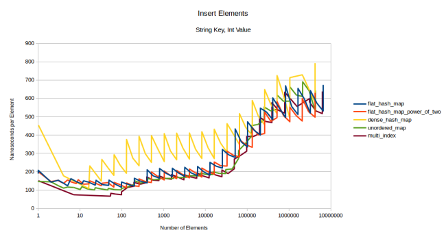
dense_hash_map is surprisingly slow in this benchmark. The reason for that is that my version of dense_hash_map doesn’t support move semantics yet. So it makes unnecessary string copies. I’m using the version of dense_hash_map that comes with Ubuntu 16.04, which is probably a bit out of date. But I also can’t seem to find a version that does support move semantics, so I’ll stick with this version.
So we’ll use this graph mostly to compare my table against the node base containers, and my table loses. Once again I blame this on the higher cost of reallocation. So let’s try what happens if I reserve first:

… Honestly, I can’t read anything from this. The cost of the string copy dominates and all tables look the same. The main lesson to learn from this is that when your type is expensive to copy, that will dominate the insertion time and you should probably pick your hash table based on the other measures, like lookup time. We can see a similar picture when I insert strings as key with a large value type:

Once again dense_hash_map is slow because it initializes all those bytes. The other tables are pretty much the same because the copying cost dominates. Except that my flat_hash_map_power_of_two has that same weird spike at exactly 16385 elements due to increased time spent in clear_page_c_e that I also had when inserting ints with a 1024 byte value.
Lesson learned from this: If you have a large type, inserts will be equally slow in all tables, you should call reserve ahead of time, and the node based containers are a much more competitive option for large types than they are for small types.
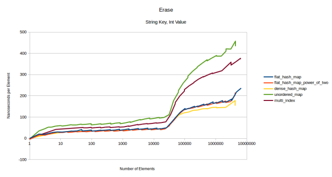
Let’s also measure erasing elements. Once again I ran three tests for ints as keys and three tests for strings as keys: Using a 4 byte value, a 32 byte value and a 1024 byte value. The four byte value picture is shown above. The 32 byte value picture looks identical, so I’m not even going to show it. The 1024 byte value picture looks like this:
The main difference is that dense_hash_map got a lot slower. This is the same problem as in the others pictures with large value types: The other tables just consider an item deleted and call the destructor which is a no-op for my struct. dense_hash_map will overwrite the value with the “empty” key/value pair which is a large operation if you have 1024 bytes of data.
Otherwise the main difference here is that erasing from flat_hash_map has gotten much more spiky than it was in the other erase picture above, and the line has moved up considerably, getting almost as expensive as in the node based containers. I think the reason for this is that the flat_hash_map has to move elements around when an item gets erased, and that is expensive if each element is 1028 bytes of data.
The graphs for erasing strings look similar enough to the graphs for erasing ints that they’re almost not worth showing. Here is one though:
Looks very similar to erasing ints. If I make the value size 1024 bytes, the graph looks very similar to the one above this one, so just look at that one again.
The final test is the “insert, erase and insert again” test I ran above where I do inserts and erases in random orders. I reduced the number to 10,000 elements because I ran out of memory when running this with ten million 1028 byte elements. It’s also much faster to generate these graphs when I’m using fewer elements. Let’s start with a 32 byte value type:
flat_hash_map actually beats dense_hash_map now. The difference gets bigger if we increase the size of the value even more:
With a really large value type my table beats dense_hash_map. However now the node based containers beat my hash table at first, but over time my table seems to catch up. The reason for this is that I’m not reserving in these graphs. So in the first insert the table has to reallocate a bunch of times and that is very expensive in the flat containers, and it’s cheaper for the node based containers. However as we erase a few elements and insert a few elements, the reallocation cost gets amortized and my tables beat unordered_map, and they would probably also beat multi_index at some point. If I reserve ahead of time they beat multi_index right away:

I actually didn’t expect this because even though I reserve ahead of time, my container still has to move elements around, and that should be really expensive for 1028 bytes of data. My only explanation for why my container remains fast is that the load factor is pretty low and that collisions are rare. When I measure this test with strings, I do see that my container slows down as expected and multi_index is competitive:
The other pictures for inserting strings look similar to the above pictures: When inserting strings with a 32 byte value type, the graph looks like this last one. When inserting with a 1024 byte value type it looks like the graphs where I did the same thing with ints as a key, both for the case where I do reserve and the case where I don’t reserve.
Performance Summary
That was quite a lot of measurements. Measuring hashtables is surprisingly complex. I’m still not entirely sure if I should measure all tables with the same load factors or with their default setting. I chose to go for the default setting here. And then there are so many different cases: Different keys, different value sizes, different table sizes, reserve or not etc. And there are a lot of different tests to do. I could have put thousands of graphs into this blog post, but at some point it just gets too much, so let me summarize:
- My new table has the fastest lookups of any table I could find
- It also has really fast insert and erase operations. Especially if you reserve the correct size ahead of time.
- For large types the node based containers can be faster if you don’t know ahead of time how many elements there will be. The cost of reallocations kills the flat containers. Without reallocation my flat container is the fastest in all benchmarks for large types.
- When inserting strings the cost of the string hashing, comparison and copy dominate and the choice of hashtable doesn’t matter much.
- google::dense_hash_map has some surprising cases where it slows down.
- boost::multi_index is a really impressive hash table. It has very good performance for a node based container.
- If you know that your hash function returns a good distribution of values, you can get a significant speed up by using the power_of_two version of my hashtable.
Exception Safety
When using my table it’s safe for you to throw exceptions in your constructor, your copy constructor, in your hash function, in your equality function and in your allocator. You are not allowed to throw exceptions in a move constructor or in a destructor. The reason for this is that I have to move elements around and maintain invariants. And if you throw in a move constructor, I don’t know how to do that.
Source Code and Usage
I’ve uploaded the source code to github. You can download it here. It’s licensed under the boost license. It’s a single header that contains both ska::flat_hash_map and ska::flat_hash_set. The interface is the same as that of std::unordered_map and std::unordered_set.
There is one complicated bit if you want to use the power_of_two version of the table: I explain how to do that further up in this blog post. Search for “ska::power_of_two_hash_policy” to get to the explanation.
Also I want to point out that my default max_load_factor is 0.5. It’s safe to set it as high as 0.9. Just be aware that your table will probably reallocate before it hits that number. It tends to reallocate before it’s 70% full because it hits the probe count limit. But if you don’t care that your table might reallocate when you’re not expecting it, you can save a bit of memory by using a higher max_load_factor while only suffering a tiny loss of performance.
Summary
I think I wrote the fastest hash table there is. It’s definitely the fastest for lookups, and it’s also really fast for insert and erase operations. The main new trick is to set an upper limit on the probe count. The probe count limit can be set to log2(n) which makes the worst case lookup time O(log(n)) instead of O(n). This actually makes a difference. The probe count limit works great with Robin Hood hashing and allows some neat optimizations in the inner loop.
The hash table is available under the boost license as both a hash_map and a hash_set version. Enjoy!

“This works great for small tables, but when I insert random values into a large table, I would get unlucky all the time and hit four probes and I would have to grow the table even though it was mostly empty.”
This wasn’t bad luck, it was just math. When your data set is large enough, you need to reconsider your definition of a rare event.
It is my understanding that hash chain length for a uniform hash follows a Poisson distribution. If you have 2^20 buckets (~ 1 million), with 2^19 element (~ 500 thousand), then you will typically have between 13-14 buckets with 6 elements in them. You will often have 1 bucket with 7 elements. As the size of your table grows, so does the magnitude of the typical worst case element. Most of the buckets in this case are still empty though (~636 thousand).
The lg(# of buckets) heuristic seems reasonable… and even safely conservative. The expected number of buckets with 20 elements in them for the previous example is 2.49*10^-19.
Thanks for doing the math on this! I knew that the probability was increasing with larger tables, but my statistics math is not that strong, so I just said “I got unlucky” so that I wouldn’t have to figure out the exact probabilities.
You’re right that log2 may be a bit conservative. I mostly arrived at it because there are several bit-twiddling hacks out there to compute it quickly. And the result of log2 is small enough that it doesn’t bother me if it’s too conservative.
On the other hand you also can’t look at buckets individually: If in a table with 500 thousand elements in it there will be 13-14 buckets with 6 elements in it and 1 bucket with 7 elements, what tends to happen is that they’re all bunched together and push each other over. So if you have two buckets with six elements right next to each other, the worst element will be 12 elements away from its ideal position.
I didn’t go into that enough. That’s the “known problem” with linear probing that I talked about at the beginning: Once a few big buckets are close to each other they grow into a single block that grows together. You’re now more likely to hit that block and even small buckets start contributing to this bunch of elements, until you got a huge block where one element is suddenly 50 slots from where it wants to be. Robin Hood hashing really helps with that because it ensures that every element is at the best possible position within that block (elements end up just ordered by their initial position) and the probe count limit prevents it from getting really bad.
Instead of modulo operation which is expensive you can use fastrange:
http://lemire.me/blog/2016/06/27/a-fast-alternative-to-the-modulo-reduction/
This should speed up you prime sized hashtable because it will eliminate branching and will use ~4 instructions per “find slot” operation.
I have looked at that in the past, but the problem is that it puts all similar elements into the same slot. For example if you just insert sequential numbers counting from 0, they will literally all hash to slot 0 if you’re on a sixty four bit platform. You have to count up to billions of elements before they start hashing to the second slot, third slot etc.
In fact I once tried using this method with numbers that were pre-hashed so that they looked random to me. But the hash function used wasn’t of very high quality so there was a pattern in the data, something like integers in the range from 0x3c000000 to 0x4c000000 were more common than other integers. And the fast range function immediately broke for me because all integers that fell into the pattern would hash to the same slot, resulting in very slow lookups and inserts for those numbers.
So I really like the fastrange idea, but you run into similar problems as when using powers of two: You have to make extra sure that there are no patterns of similar integers in the outputs of your hash function.
So I agree that it’s a great optimization sometimes, but I don’t want to use it by default.
Another example of similar approach is https://github.com/larytet/emcpp/blob/master/src/HashTable.h
Limited number of collisions, resizing automatic or on demand, fast hash function, a simple array bind the hash.
P.S. Please ignore the link above – it is not really relevant.
please add readme files in your repositories!
>std::unordered_map [is] self-explanatory.
Not quite 🙂 Since there are different implementations of std::unordered_map (libstdc++, libc++, MSVC’s C++ standard library…)
Sorry, you’re right. This one is the GCC unordered_map. That being said I have worked with the GCC unordered_map and with the Microsoft unordered_map, and they both had similar performance. (that being said I also know that Microsoft did some updates to their unordered_map since then so I might be out of date)
I think that a good implementation of std::unordered_map could be as fast as boost::multi_index. So you can look at that one as a representation of an ideal node based container if you want to.
As a libc++ maintainer I would love to see the graphs with libc++ included. I’ve done a lot of work to optimize our implementation and I suspect it will perform differently than libstdc++. Hopefully it would prove to be a “good implementation” 🙂
Nice work! What about an attacker constructing a request that invokes table growth with each single insert? Once you get that covered well and can also set a linear worst case boundary on the growth, this table is cool. Btw, without bounding the growth under attack, your worst case performance will be terrible (because an attack is just a worst case), so I think you might want to do all those analysis a bit more in-depth.
Right, that’s what I meant when I talked about the “new attack” in the paragraph about security concerns: You can easily make the computer run out of memory by inserting intentionally bad data into the table.
That being said this does not affect the worst case for lookups. Lookups will actually be very fast in this case because the table is mostly empty. This only affects the worst case for inserts, which you can make really slow with malicious data.
Well done.
PS: It’s Robin Hood hashing. https://en.wikipedia.org/wiki/Hash_table#Robin_Hood_hashing
It’s really interesting how actually a cache miss could have multiple implications having different implementations. But I think I’m getting something wrong, in case you know for example for what are you looking, isn’t it O(1), why should you go to O(log(n)) in that case for a lookup when you know the key for example?
Yes, it’s O(1) in the average case. It’s O(log(n)) in the worst case. Other hash tables are O(1) in the average case, but O(n) in the worst case.
So I only talked about the worst case because that’s the only thing that changed. But when using this you should use it as if lookups were O(1). Otherwise there would be no point to hash tables and you would use std::map.
I don’t think this is correct. Sure it’s O(log(n)) in the worst case, but only if n = the hash table capacity. Normally when we say hash tables are O(n) in the worst case, we mean n = number of elements present. In the worst case your hash table capacity = 2**elements, so I think it’s more accurate to say your worst-case lookup is O(log(capacity)) = O(log(2**elements)) = O(elements), just like other hash tables.
@Nathaniel: My capacity is 2*elements, not 2^elements. So it’s just O(log(2*elements)) which is just O(log(elements)).
Sure, if you don’t have too many collisions. But we’re talking about worst cases. Worst case is when all the elements have the same hash, in which case your table is indeed 2^elements, and lookups are O(elements).
Heh, yeah I hadn’t thought about that case. Yes, if you have really bad data and all the keys hash into the same bucket, you’ll get O(n) lookup time. However you’re going to run out of memory really quickly. Since I allocate more than 2^n memory, that n can at most go up to 64. So it’s O(n) for n < 64. If you have more than 64 elements in your table, it's O(log(n)).
Or to put it another way: My hashtable detects really slow cases and tries to "save itself" by reallocating. If the input data is really bad so that even after reallocating all the keys hash to the same value, that trick won't work. Most of the time it will work though and then my hash table will be faster than others.
Have you compared to khash?
I have now 😀
khash is interesting. It’s also very fast and would probably merit its own detailed comparison like I did for dense_hash_map above. But just running my first “successful lookup” and “unsuccessful lookup” benchmarks I get these graphs:
So it looks like it can be faster in some situations and slower in others. But my hash table in its power of two version seems to beat it on average.
Khash also has a few interesting tricks up its sleeve. For example it generates different code for 32 bit keys than for 64 bit keys. My table does not give you that choice: It’s always whatever your size_t is.
(oh and if the pictures of the graph don’t work, bear with me. Trying to figure out how to insert pictures into comments)
You can solve the distance_from_desired (byte) alignment issue without needing to touch more cache lines.
Separate the payload and distance_from_desired and put them to the same cache line.
Example: Unsigned int (4 byte) payload
Current mem layout (per cache line):
8 x {unsigned int payload, byte distance, 3 bytes padding} = 64 bytes
Separated mem layout (per cache line):
12 x unsigned int payload = 48 bytes
12 x byte distance = 12 bytes
= total 60 bytes
= 50% more elements per cache line
Example: Pointer (8 byte) payload
Current mem layout (per cache line):
4 x {pointer payload, byte distance, 7 bytes padding} = 64 bytes
Separated mem layout (per cache line):
7 x pointer payload = 56 bytes
7 x byte distance = 7 bytes
= total 63 bytes
= 75% more elements per cache line
These are significant improvements with probe size of 10. The probability to touch two cache lines instead of one decrease a lot. Also the hash table becomes more dense, meaning that the probability to find existing data in L3 cache increases (further improving performance). Most of additional indexing math should be performed at compile time (template type is known at compile time).
That’s a great idea. Thanks!
I probably won’t get to try that optimization this week, but I’ll try to get to it soon.
Did you manage to test this already? I’d love to read a follow up post, keep up the good work!
Great writeup! I’ve recently spent quite some time implementing a robin hood based hashmap as well. Could you run a comparison with that as well?
https://github.com/martinus/robin-hood-hashing/blob/master/src/RobinHoodInfobytePairNoOverflow.h
I have a much improved implementation that I unfortunately cannot share. But I’d like to share some of the tricks that are also very important for a fast general purpose implementation:
* Use lazy initialization: Don’t allocate anything as long as the hashmap stays empty. Only allocate stuff when the first element is inserted. This can enormously speed up the creation of maps
* For robin hood map to be fast it is very important that swap() is fast. This is only the case with simple values. I have an implementation that at compile time switches to a node-based implementation when sizeof(mapped_type) > 2*sizof(void*). The advantage is that swap will be very fast again because only a pointer is exchanged, the disadvantage is that it requires lots of allocations.
* For the node based implementation, I use a pool allocator. Whenever a node is free’d, I reuse that node’s memory as a pointer in a linked list of available memory. That way you pay the allocation penalty only once per node.
* I really like the idea of using an offset byte, as in the hashmap that I’ve linked above. That way much less key comparisons are required, which is important if you e.g. have an std::string as the key. Also I believe it is much better for cache locality: when looking for an entry in a map that is quite full, you mostly check byte for byte of the index map, and then compare only the relevant keys.
It would be nice to add some more maps to the tests because it doesn’t seem to be the fastest one.
I took the k-nucleotide test which has a heavy read load on a hash map (http://benchmarksgame.alioth.debian.org/u64q/program.php?test=knucleotide&lang=gpp&id=3) and changed the `unsigned N = sysconf (_SC_NPROCESSORS_ONLN);` to `unsigned N = 1;` to make it runs on one core only.
g++ -O3 -std=c++14 knucleotide.cpp -o knucleotide -lpthread
time ./knucleotide < input25000000.txt
__gnu_pbds::cc_hash_table: 0m18.297s
std::unordered_map: 0m38.767s
tsl::hopscotch_map (seems to do well from a post on reddit): 0m19.288s
ska::flat_hash_map: 0m25.177s
ska::flat_hash_map power of two: 0m24.454s
Couldn't make it work with google::dense_hash_map.
That is a very interesting test. I also get your results when I run it. The main thing it tests is how long a successful lookup takes, and that is what I claim to be very good at. So it’s not good to see that I’m not winning.
Looking at the disassembly, it seems to mostly come from a series of slightly awkward assembly. For example the assembly for the hash function looks worse when using my hash table than when using __gnu_pbds::cc_hash_table. That code is completely independent of the chosen hashtable though. One reason for the worse assembly might be that my operator[] function is much bigger, so more code got inlined and the optimizer got confused because there is just too much code at once. I’ll try to make its job easier by splitting my operator[] function in two so that the fast case of the key already existing can be inlined separately from the slow case of the key not existing. After that there are some more small awkward choices that I made in my table that I should be able to optimize. For example my method for masking off the bottom bits generates more instructions than it does in other tables.
I think this is mainly a case of me only optimizing until I was faster than google::dense_hash_map. Now that I have a benchmark where I’m not the fastest, I can do some more optimizations.
I’ll also see if I can optimize the benchmark overall. What kind of language benchmark has Rust as 30% faster than C++? At worst C++ should be equal in speed…
I’ll get back to you by next week.
So I think I have a new fastest implementation. It’s uploaded at
https://github.com/skarupke/knucleotide
It’s faster than Rust. You can also switch to use the cc_hash_table in there, and sometimes that one beats my hash table. I don’t know why that is. If I run the code in google benchmark my table wins pretty easily. If I run it as a standalone executable the cc_hash_table wins.
Specifically the fastest time I have measured is with the cc_hash_table. But on average mine is faster. Meaning the cc_hash_table has better positive outliers. So for example my table will take between 4.4 seconds and 4.5 seconds on my machine. The cc_hash_table will take between 4.5 seconds and 4.6 seconds. But every once in a while it will take 4.3 seconds.
Since I only see that when running as a standalone executable, and I don’t see it when running as part of google benchmark, I have to assume that it’s something with starting a new executable. Maybe something with a fresh memory manager. Maybe it doesn’t like that my hashtable requests large chunks of memory instead of small allocations. That seems unlikely though. I literally have no idea where the difference comes from.
So my result is:
– My hashtable is fastest in knucleotide when measuring in google benchmark.
– It’s also faster on average than cc_hash_table when measuring as a standalone executable.
– However I get the fastest measurements when using cc_hash_table.
– When using my hashtable or cc_hash_table, I always beat Rust.
I’ll try submitting it to the website.
Oh and when running in Google Benchmark my hash table takes between 2.4 seconds and 2.5 seconds, and cc_hash_table takes between 2.7 seconds and 2.9 seconds. There is large difference, and cc_hash_table never beats my hash table.
The google benchmark code doesn’t measure how long it takes to read the inputs from disk, but that should take the same amount of time independent of hash table.
Thank you for your answer.
Effectively it’s faster with this new knucleotide benchmark, but I tried the last version of ska::flat_hash_map with power of two size on the original benchmark and I still get a large difference for this case (just reduced to 0m23.074s, still 25% slower).
Do you know why there is such a difference on the original test?
I don’t quite know. What happens is that the assembly looks slightly worse when compiling with my table than when compiling with the other table. For example in this function:
   void reset(const std::string& s,unsigned beg,unsigned end)
   {
      size = end-beg;
      data = 0;
      for(unsigned i = beg; i != end; ++i)
      {
         data <<= 2;
         data |= tonum[unsigned(s[i])];
      }
   }
The compiler will spill the “data” variable from a register into memory and then read it back from memory. In every single loop iteration. It doesn’t do that when using the other hashtable. So when using cc_hash_table the program spends roughly 24% of its time in this loop, when using my hash table it spends roughly 28% of its time in this loop.
What’s weird is that the hash table is not used in this loop. That “tonum” variable in the middle there is a normal array look up. Since this loop is completely unrelated to the hash table I have no idea why the compiler generates different assembly.
The fix is to store data on the stack and to only write it back to the member variable at the end of the loop, like this:
   void reset(const std::string& s,unsigned beg,unsigned end)
   {
      size = end-beg;
      uint64_t new_data = 0;
      for(unsigned i = beg; i != end; ++i)
      {
         new_data <<= 2;
         new_data |= tonum[unsigned(s[i])];
      }
      data = new_data;
   }
Similarly in this function:
HashMap calculate(const std::string& input,unsigned size, unsigned beg=0,unsigned incr=1)
{
   HashMap frequencies;
   T tmp;
   for (unsigned i = beg, i_end = input.size() + 1 - size; i < i_end; i+=incr)
   {
     tmp.reset(input,i,i+size);
      ++frequencies[tmp];
   }
   return frequencies;
}
The “tmp” variable is also being spilled to the stack and read back every iteration. In this case I know why that is: when using operator[] in the hash table the fast case is that the item already exists in the table, and no new element has to be inserted. The slow case is that the element does not exist. If the table hits the slow case, it calls a function and passes the tmp variable as a reference to that function. And in theory that function could modify that reference, so it has to be read back before its used again.
This doesn’t seem to happen with the other hash table because in that hash table the compiler doesn’t put the slow case and the fast case together. They get compiled separately so that there is one path through the loop where the variable does have to be stored to the stack and read back, and there is one path through the loop where it does not. No matter what I try I can’t get the compiler to do this for my table.
Instead I optimized this by passing a copy of tmp to the operator[]. For some reason it still gets stored to the stack, but at least it doesn’t get read back.
So basically if I want to make them similarly fast, I end up having to do all the optimizations that I did. I just have to undo clumsy assembly one bit at a time.
What is the reason for this clumsy assembly? I honestly don’t know. As far as I can tell the compiler should use the same number of registers for both hash tables. The assembly really looks very similar:
1. Compute the hash
2. Read the m_mask member from the table
3. Apply the mask
4. Get the m_entries pointer from the table
5. Add the result of step 3 to the result of step 4
6. Read the entry
7. Check if its valid
8. Compare the key in the entry, check if its equal
9. Increment the value
The only real difference is in step 7. In cc_hash_table that check involves doing a nullptr comparison. In my hash table that involves checking whether a single byte is greater or equal to 0. Otherwise there are small differences in assembly in many of these steps (for example step 5 requires multiplying the mask by 24 for my table, and multiplying it by 8 for cc_hash_table) but nothing that should make it have to use more registers or otherwise lose performance.
On the other hand I have stared at enough assembly for now. I’m kinda done with this benchmark.
A potential solution for the padding without additional cache misses is that you could alternate data and metadata bytes inside each cache line. For example, with a 64 byte cache line, with T being 8 bytes and 8 byte aligned, you could have 7 T’s followed by 7 bytes, which would only waste 1/64 instead of 7/16.
> I’ll also see if I can optimize the benchmark overall. What kind of language benchmark has Rust as 30% faster than C++? At worst C++ should be equal in speed…
That might be the result of benchmarking GCC vs LLVM. Nowadays they are almost on par, 30% difference in some microbenchmark looks feasible to me.
If you want to compare the implementations you should benchmark the Rust code vs the C++ compiled with clang++. If there are any differences, I expect that one can remove them by just tunning the slower implementation a bit. (Note also that in Rust pointers/references have almost always a `__restrict` annotation because they cannot alias mutably, so adding this annotation to the C++ code might resolve the issue).
I still haven’t gotten around to the promised improvement, but just from looking at the source code you can see that the two implementations have different speeds simply because they use a different algorithm: The Rust version uses an incremental hash function, the C++ version does not. That alone can account for all of the difference: In the last benchmark in there which has to hash an 18 character string, the C++ version will start from scratch and re-hash the 18 characters for every loop iteration. The Rust version only updates the hash with one new character for the loop iteration.
Apparently someone already suggested my idea but I hadn’t read all the comments yet.
Anyways, another observation that hasn’t been mentioned yet is that there is no reason that the key and value have to be allocated together other than the antiquated notion that maps should be sets with a pair as the value type. If the interface were changed to not use a pair, the implementation could store large values separately from keys and therefore, not have a performance penalty for storing large values.
It is startling/disappointing that a generic a%b is so slow that a switch with various a%C beats it handily.
switching via an array of function pointers seems to be faster still:
size_t modf_0(size_t hash) { return 0llu; }
size_t modf_1(size_t hash) {return hash % 2llu; }
…
size_t (*modfp[])(size_t) = { modf_1, modf_2, … };
#define index_for_hash(hash) modfp[prime_index](hash)
Something like that.
That’s a good idea and it doesn’t even take any extra storage. I’ll try it. Thanks!
Oh, and this post claims that the interface is the same as boost::unordered_map, but it doesn’t allow iterating over buckets.
std::unordered_map (based on boost::unordered_map) is woefully overspecified, especially 23.2.5 [unord.req]/9:
The elements of an unordered associative container are organized into buckets. Keys with the same hash code appear in the same bucket. The number of buckets is automatically increased as elements are added to an unordered associative container, so that the average number of elements per bucket is kept below a bound. Rehashing invalidates iterators, changes ordering between elements, and changes which buckets elements appear in, but does not invalidate pointers or references to elements. For unordered_multiset and unordered_multimap, rehashing preserves the relative ordering of equivalent elements.
Not invalidating pointers to the elements means that an even remotely fast hash table can’t really be achieved on modern hardware.
The bucket iterators are pretty easy to support. One artifact of Robin Hood linear probing is that it stores all elements in a bucket together. So I could easily find the beginning and end iterators for a bucket. I don’t know what they’re for though. Why do you want to iterate over buckets? I didn’t add the feature because it seemed to not make sense.
Similarly my iterators are forward iterators only. The ones on unordered_map are bidirectional. There is a cost to supporting bidirectional iterators and I don’t see the use case. Why do you care whether you iterate over an unordered list forward or backward?
There are also some allocator features that I don’t support. The main reason there is that they looked complicated.
I would of course support all of these features if somebody needs them. So if you need to be able to iterate over buckets, let me know.
I doubt you would support the iterator invalidation guarantees that the standard wants. The standard requires that inserting an element into an unordered_map doesn’t invalidate any other iterators. That pretty much rules out an open-addressing scheme and forces a node-based implementation.
Me! I definitely want to iterate over buckets, since I am using hashtables in a mark/sweep garbage collector, and the sweep phase very much needs to iterate over every entry in the table to check the mark bit and remove (and possibly finalize) the dead ones. In fact, this has been a limiting factor in our implementation. (And there are multiple such tables; these aren’t core to the GC algorithm, they’re any application table keyed off of a GCed object.)
My belief is that the load factor is very important for this, because if you have a load factor of 0.5, then your branch predictor is completely useless; it’ll guess wrong very close to half the time. I haven’t tested it rigorously, though.
It would be interesting if you could test how the performance of your hash table varies if you increase the lookup bound to, e.g., 1.2 * log2(n), or other similar values, with a higher maximum load factor. Some applications are memory bound, so achieving a higher load factor in practice would be good, especially if your bounded search idea still keeps the performance good. Maybe you can tweak the constant to achieve a range of load factors up to around 0.9. Speed could even be improved, since more would fit in cache.
It actually wouldn’t make much of a difference because you hit the bad cases very rarely. Your average lookup won’t hit the limit.
I would pick a nice round number like 2 * log2(n). The biggest downside with doing that is that you have to allocate more extra space at the end of the array. Otherwise I have to add bounds checking.
It’s certainly worth trying. I would want to name it something different though. Like google has a sparse_hash_map and a dense_hash_map where the dense one uses more memory but is faster.
That being said I may not do this because I kinda want to move on from this hashtable thing.
Would definitely attend a talk about this. Would be great content for CppCon!
I’m actually going to give a talk at C++Now about my sorting algorithm. (https://probablydance.com/2016/12/27/i-wrote-a-faster-sorting-algorithm/)
It’s going to be my first talk ever. Depending on how that goes I might give more.
Already done at cppcon 2016 (https://www.youtube.com/watch?v=aXj_DsIx1xs, https://github.com/tjizep/rabbit). Rabbit hashing uses the “novel” feature of this hash table – a fixed probe length (configurable to either constant length or log table size) – but it uses straight linear hashing with an overflow bucket rather than robin hood hashing – and has a different concept for collision and deletion detection.
Would be interesting to see a performance comparison.
The division by prime can be replaced with inverse multiplication not by compiler, but in runtime, precalculating when a next table size is selected. For example, https://github.com/ridiculousfish/libdivide provides this, and I’m sure there are simpler others.
Notice russian translation of your post: https://habrahabr.ru/company/mailru/blog/323242/
discussion directions are somewhat different.
I think libdivide doesn’t have a modulo operator. Of course once you have division, you could make your own modulo operator. Which I think is essentially what GCC does for large primes. But the compiler has a few more tricks and the custom assembly is probably faster than using libdivide.
Using libdivide would make sense if I didn’t have a fixed list of prime numbers though.
For the russian translation: I think it’s OK to translate the blog post, but they really should give credit and link back to the original.
> I think libdivide doesn’t have a modulo operator.
Nor AArch64 has, for example. Only quotient is exposed by a hardware; then, the remainder can be easily found (and they provide integer(!) fused-multiply-and-add for this).
> Using libdivide would make sense if I didn’t have a fixed list of prime numbers though.
Yep, but you have to provide not only list of them in your source (as e.g. GCC STL does) but also code to apply them. It isn’t complex, but rather cumbersome. Also, compiler intelligence for sparse set select {} isn’t very predictable. GCC generates a binary tree of compares and conditional branchings. A series of 5-7 branches, even if all predicted, is generally slower than a single sequence of multiply-and-shifts. Finally, you can extract only a small subset of its actions (as for uint32_t). Anyway, this needs measuring in a real setup.
> but they really should give credit and link back to the original.
They did, but that’s a known issue of habrahabr engine: link to original is very counter-obvious. Just after the main text but before comments, find the line:
>> Автор: @AloneCoder Malte Skarupke
your name field is also the hyperlink to the original article.
Is it the same like this?
http://martin.ankerl.com/2016/09/15/very-fast-hashmap-in-c-part-1/
It looks like that implementation uses a different trick. I don’t think it’ll be as fast, but I would have to do run benchmarks to be sure. Sorry, can’t tell you any more right now.
Hi Malte, would it be possible to get a copy of your benchmark code? I’ve been working on a slightly different robin hood implementation of my own and it would be nice to compare my version to yours.
Hi, sorry for the long delay in responding.
The benchmark code is not in a good state at all. But I’ve uploaded it here:
https://probablydance.files.wordpress.com/2017/08/hashtable_test_and_benchmark_code.zip
Also read my comment in response to Matthew Kulukundis below, which has a bit more of a description.
Sorry if you cover this somewhere else, but are your benchmarks and graphing code available as well? I would like to try and reproduce your results.
It’s not high quality code, but I’ll try to find a way to upload it. For the graphing I actually just manually copy+paste my results to a table in Libre Office and use their graphing functionality.
I’ve uploaded a copy of my code here:
https://probablydance.files.wordpress.com/2017/08/hashtable_test_and_benchmark_code.zip
It’s a qt creator project. I can’t promise that it will run or that it will be easy to get to run. Also there is a lot of junk in there, including half-finished hash tables and half-working test frameworks from boost and abandoned benchmark code that I copied from other developers. Also I don’t know what license this should be under, because it’s code copy+pasted together from a bunch of places, so don’t distribute it too much.
All the actual benchmark code is in the file profiling/unique_scattered_lookup.cpp. You can probably ignore most other files in there, but I honestly don’t know for sure right now.
Oh and sorry for the long delay in responding.
Can you please post instructions on how to replicate your benchmarks? Thanks!
Hi, sorry for the long delay in responding. I uploaded the code here:
https://probablydance.files.wordpress.com/2017/08/hashtable_test_and_benchmark_code.zip
And I gave a bit more of a response to Matthew Kulukundis above. But be warned: the code is not in a good state. It was never intended to be published.
The graphs aren’t exactly fair without considering the extra space required for the distance_from_desired. If the competitors used that space for a slightly larger table, they’d do a little better. I was thinking you could account for this by tweaking the max_load_factor, without needing to touch the max probe count? Hm.
Though in my case, I really want a high max_load_factor to speed up iteration, I’d think at least 0.9. Which means I need to increase the max probe count, I guess.
If you look around on the FreeBasic forum there is a way to keep track of the displacements using a histogram.
I responded on to Matthew Kulukundis on YouTube where he did a presentation, not sure if it is a similar implementation, but the idea I have is generic enough for you to play with.
The generic idea:
* Have a primary hash table without any load factor at all.
* Each input is projected to be present in some bucket/group.
* If it cannot be found in that specific bucket/group (or any ** fixed number ** of them as you tune it), switch the operation to a more “conventional” second level structure.
What this gets us:
* The L1 hash table can be completely filled (no more load-factor directed sizing).
* Lookup in the L1 hash becomes a fixed number of steps, great for code optimization.
* When the L1 grows in powers of two (as many do), then having a smaller L2 to deal with collisions in L2 can save a ton of memory vs growing the L1.
Notes:
The L2 still operates with a load-factor and could even resize independently from the L1.
As a growth policy consider resizing the L1 instead of resizing L2 only when:
* L2 size starts to look too much like a L1 on its own (say over 1/16th for large tables);
* L2 gets hit too often in operations vs L1 Level one hits (run-time statistics).
With run-time statistics, an optimized load-factor for the L2 can probably computed during resizing operations.
Not that resizing the L2 only, involves moving less data, which is good. It does only re-distribute the collisions in L1 which remain in-place until a L1 growth.
I hope this all makes sense 🙂
Oh, and for every small tables, L2 can be considered the L1, bypassing the L1 entirely.
Hi Malte have you seen: https://lemire.me/blog/2016/06/27/a-fast-alternative-to-the-modulo-reduction/
as an alternative to powers of 2 for N
Funny you should ask that, I just wrote a blog post about a better alternative to it:
I mention it briefly in there under the name “fasthash”.
There is also that https://libdivide.com/ that makes division operation much faster.
Hello Malte,
I want to use flat_hash_map as a database. Is there a way to make it persistent? I want to store the map on disk and load it again to query it or insert further items. Is there example code for that purpose or could you point me to the right direction?
There isn’t any built-in way to do that. And I am not sure if I’d want to provide one because then all future versions would have to store things in the same order internally, and that’s a limitation I’m not sure I want to put on myself at this point.
But it’s pretty easy for you to write this yourself: Just iterate through all items and persist them to disk one at a time. And when loading load them in and add them to the map one at a time. If you write out the size of the map beforehand, you can also call reserve() to make it faster. If you write the code generically, it should be the same code for all hash tables, not just for mine.
Thank you very much for your reply!
For the sequential inserts, Im slightly confused how Robin hood takes a long time to decide an element ‘x’ is not in the table. Shouldn’t the linear probe look at the probing slot and decide, because the second element ‘y’ is in its proper spot, that x cannot possibly be in the table (because it would have pushed y out of its spot?). I may be misunderstanding. Great read!
Sadly this algorithm and code is unapproachable for me as i dont understand a line of C++, hopefully if you have to time can you port it to C?
Probably not. I can read C, but I don’t know what a hash table would look like in C. Do you only allow people to insert pointers? Or do you allow them to specify the size of the data that they want to insert? I can’t even imagine how to write a general purpose hash table without templates.
The go-to open source C hash table, uthash has users inject a “hash handle” member into their structs and use macros to access their tables (the library types themselves are concrete).
Less readable than flat_hash_map.hpp IMO (though that’s not the macros’ fault, oddly enough) and less generic than C++ containers (though one *could* probably make this more generic by wrapping contained types in struct ##typename_HASHED generated by the library, not that I’ve thought it through properly).
(Not seconding OP’s request, just posting for information purposes)
I think given the numerous differences and outright incompatibilities between flat_hash_map and std::unordered_map you shouldn’t advertise it as having the same interface, when the interfaces are, in fact, only superficially compatible (it might compile, but cause corruption in numerous ways).
For example, we had this very old and clumsy, but nevertheless correct code:
// iterate through map via iterator i, and occasionally delete like this:
auto prev = *i++;
ht.erase (prev);
This is correct code with unordered_map, but causes corruption with flat_hash_map, because it doesn’t have the same iterator stability guarantees as std::unordered_map, and obviously itertaor invalidation rules are a very important part of the interface.
This was very hard to track down (as iterator invalidation bugs often are) because it caused action at a distance only much later when the libc malloc found its chains corrupted.
So I can only strongly warn against treating flat_hash_map as a replacement for unordered_map – it is incompatible at a very deep and subtle level and can cause all kinds of corruption with otherwise correct code.
On the positive side, we found flat_hash_map to be nice to use and indeed very fast and versatile.
However, replacing our existing hash table code by using flat_hash_map caused a lot of corruption and pain until we ironed out the incompatibilities, and this left a bad taste for us: if you misrepresent something as basic as interface compatibility, what else of what you wrote can we trust?
I think removing the wrong and misleading claims of compatibility to std::unordered_map will be a win-win for everybody, without diminishing the usefulness of your work.
The idiom you are suggesting should work (and has been tested). Are you sure you are not hitting a different issue?
We are extremely careful in the claims we have made and have already converted about 60% of Google’s existing code base.
Can you post a full repro for this? The pattern you are suggesting definitely should work (and is tested).
I have learned your code, and found there is a bug in emplace_new_key() at line 824 flat_hash_map.hpp? I’m not sure, pls help to check. https://github.com/skarupke/flat_hash_map/issues/23
@skarupke, i have a idea about handling the case of the allocator throwing. please see my comment on github. https://github.com/skarupke/flat_hash_map/issues/23
Consider this: Robin hood hashing with linear probing essentially is sorting the entries by the hash value of the key when collisions occur. Therefore lookup can be accelerated with interpolation search, when the probe sequence is high, on the order of 8.
Expanding on this idea I developed hash table optimized for high load factors, connecting sorted arrays with hash tables.
https://drive.google.com/file/d/1rLgtoubKnubigPLKL96TEPZSoAgpijzw/view
https://github.com/1ykos/ordered_patch_map
New links:
https://github.com/1ykos/patchmap
https://1ykos.github.io/patchmap/
Hi Malte,
are you aware of fastest (known to me) way of lookuping – my duo: FNV1A-Yorikke + Btrees order 3?
Could you also add this hash_map in your comparison: https://github.com/hordi/hash
For next simplest comparison I have interesting enough results, it would be good to run actual and full tests.
#include “flat_hash_map.hpp”
#include “hash_set.h”
#include <Windows.h>
class Timer
{
public:
Timer(const char* msg) :_msg(msg), _start(GetTickCount()) {}
~Timer()
{
DWORD end = GetTickCount();
printf(“time(%s): %u\n”, _msg, (unsigned)(end – _start));
}
private:
const char* _msg;
DWORD _start;
};
const size_t MAX_ELEMENTS = 1000000;
template
static void insert(T& m)
{
Timer t(“insert”);
}
template
static void erase(T& m)
{
Timer t(“erase”);
}
template
static void find_erase(T& m)
{
Timer t(“find_erase”);
}
template
static size_t find(const T& m)
{
size_t ret = 0;
}
template
static size_t find_back(const T& m)
{
size_t ret = 0;
}
template
static size_t test(T& m, const char* name)
{
puts(name);
}
int main()
{
ska::flat_hash_map<size_t, size_t> m0;
hash_map<size_t, size_t> m1;
}
ska::flat_hash_map
time(insert): 484
time(erase): 47
time(insert): 328
time(find_erase): 62
time(insert): 329
time(find): 812
time(find_back): 828
hash_map
time(insert): 375
time(erase): 31
time(insert): 344
time(find_erase): 16
time(insert): 344
time(find): 390
time(find_back): 391
…and here I set out to learn how to make a hash table so I could try to make one faster than the STL. You’ve done a ton of useful work here! This hash table is nuts. 800k+ lines from an input file, parsed to a key and string data to compare to another 800k+ line input file. Streamed the 2nd input file to compare to the hash table. Needed both to insert data and lookup data to get it done. Looking for changed data and missing keys in the second file. From your data, it looks like the other methods get exponentially slower for the most part and your table stays pretty steady. Love it! Thanks for the help! Shaved about 15% off the std::unordered_map time.
Not sure if this is still active/considered the fastest but I think I wrote one faster.
If your interested the code is at: https://github.com/goldsteinn/hashtable_test
Either way your post inspired me to write it and I learned a lot doing so 🙂
Do you have benchmarks with random 64bit keys somewhere?
That benchmark has option for 64 bit random keys. Worth noting I’ve rewritten it use if your going to benchmark my table use: https://github.com/goldsteinn/unordered_map just include “fht_ht.hpp”. It has about the same api as standard unordered map.
Very interesting article.
However, I see a problem that is unlikely to happen for random data, but may happen with bad hash function or malicious input.
Say you want to limit look ups to N, but you get N+1 items all with the same hash.
If I understand the code properly, it will try to rehash the table, but it will not help. So it calls rehash() recursively until it runs out of memory.
The same may also happen when using powers of 2 if there are N+1 items that differ only in high hash bits that are not used for calculating the bucket.